


Just as we can model a road map as a directed graph in order to find the shortest path from one point to another, we can also interpret a directed graph as a "flow network" and use it to answer questions about material flows. Imagine a material coursing through a system from a source, where the material is produced, to a sink, where it is consumed. The source produces the material at some steady rate, and the sink consumes the material at the same rate. The "flow" of the material at any point in the system is intuitively the rate at which the material moves. Flow networks can be used to model liquids flowing through pipes, parts through assembly lines, current through electrical networks, information through communication networks, and so forth.
Each directed edge in a flow network can be thought of as a conduit for the material. Each conduit has a stated capacity, given as a maximum rate at which the material can flow through the conduit, such as 200 gallons of liquid per hour through a pipe or 20 amperes of electrical current through a wire. Vertices are conduit junctions, and other than the source and sink, material flows through the vertices without collecting in them. In other words, the rate at which material enters a vertex must equal the rate at which it leaves the vertex. We call this property "flow conservation," and it is the same as Kirchhoff's Current Law when the material is electrical current.
The maximum-flow problem is the simplest problem concerning flow networks. It asks, What is the greatest rate at which material can be shipped from the source to the sink without violating any capacity constraints? As we shall see in this chapter, this problem can be solved by efficient algorithms. Moreover, the basic techniques used by these algorithms can be adapted to solve other network-flow problems.
This chapter presents two general methods for solving the maximum-flow problem. Section 27.1 formalizes the notions of flow networks and flows, formally defining the maximum-flow problem. Section 27.2 describes the classical method of Ford and Fulkerson for finding maximum flows. An application of this method, finding a maximum matching in an undirected bipartite graph, is given in Section 27.3. Section 27.4 presents the preflow-push method, which underlies many of the fastest algorithms for network-flow problems. Section 27.5 covers the "lift-to-front" algorithm, a particular implementation of the preflow-push method that runs in time O(V3). Although this algorithm is not the fastest algorithm known, it illustrates some of the techniques used in the asymptotically fastest algorithms, and it is reasonably efficient in practice.
In this section, we give a graph-theoretic definition of flow networks, discuss their properties, and define the maximum-flow problem precisely. We also introduce some helpful notation.
A flow network G = (V, E) is a directed graph in which each edge (u,v)
We are now ready to define flows more formally. Let G = (V,E) be a flow network (with an implied capacity function c). Let s be the source of the network, and let t be the sink. A flow in G is a real-valued function f: V x V
Capacity constraint: For all u, v
Skew symmetry: For all u, v
Flow conservation: For all u
The quantity â (u, v), which can be positive or negative, is called the net flow from vertex u to vertex v. The value of a flow f is defined as
that is, the total net flow out of the source. (Here, the |
Before seeing an example of a network-flow problem, let us briefly explore the three flow properties. The capacity constraint simply says that the net flow from one vertex to another must not exceed the given capacity. Skew symmetry says that the net flow from a vertex u to a vertex v is the negative of the net flow in the reverse direction. Thus, the net flow from a vertex to itself is 0, since for all u
for all v
Observe also that there can be no net flow between u and v if there is no edge between them. If neither (u, v)
Our last observation concerning the flow properties deals with net flows that are positive. The positive net flow entering a vertex v is defined by
The positive net flow leaving a vertex is defined symmetrically. One interpretation of the flow-conservation property is that the positive net flow entering a vertex other than the source or sink must equal the positive net flow leaving the vertex.
A flow network can model the trucking problem shown in Figure 27.1. The Lucky Puck Company has a factory (source s) in Vancouver that manufactures hockey pucks, and it has a warehouse (sink t) in Winnipeg that stocks them. Lucky Puck leases space on trucks from another firm to ship the pucks from the factory to the warehouse. Because the trucks travel over specified routes between cities and have a limited capacity, Lucky Puck can ship at most c(u, v) crates per day between each pair of cities u and v in Figure 27.1 (a). Lucky Puck has no control over these routes and capacities and so cannot alter the flow network shown in Figure 27.1(a). Their goal is to determine the largest number p of crates per day that can be shipped and then to produce this amount, since there is no point in producing more pucks than they can ship to their warehouse.
The rate at which pucks are shipped along any truck route is a flow. The pucks emanate from the factory at the rate of p crates per day, and p crates must arrive at the warehouse each day. Lucky Puck is not concerned with how long it takes for a given puck to get from the factory to the warehouse; they care only that p crates per day leave the factory and p crates per day arrive at the warehouse. The capacity constraints are given by the restriction that the flow â(u, v) from city u to city v to be at most c(u, v) crates per day. In a steady state, the rate at which pucks enter an intermediate city in the shipping network must equal the rate at which they leave; otherwise, they would pile up. Flow conservation is therefore obeyed. Thus, a maximum flow in the network determines the maximum number p of crates per day that can be shipped.
Figure 27.1(b) shows a possible flow in the network that is represented in a way that naturally corresponds to shipments. For any two vertices u and v in the network, the net flow â(u, v) corresponds to a shipment of â(u, v) crates per day from u to v. If â(u, v) is 0 or negative, then there is no shipment from u to v. Thus, in Figure 27.1(b), only edges with positive net flow are shown, followed by a slash and the capacity of the edge.
We can understand the relationship between net flows and shipments somewhat better by focusing on the shipments between two vertices. Figure 27.2(a) shows the subgraph induced by vertices v1 and v2 in the flow network of Figure 27.1. If Lucky Puck ships 8 crates per day from v1 to v2, the result is shown in Figure 27.2(b): the net flow from v1 to v2 is 8 crates per day. By skew symmetry, we also say that the net flow in the reverse direction, from v2 to v1, is -8 crates per day, even though we do not ship any pucks from v2 to v1. In general, the net flow from v1 to v2 is the number of crates per day shipped from v1 to v2 minus the number per day shipped from v2 to v1. Our convention for representing net flows is to show only positive net flows, since they indicate the actual shipments; thus, only an 8 appears in the figure, without the corresponding -8.
Now let's add another shipment, this time of 3 crates per day from v2 to v1. One natural representation of the result is shown in Figure 27.2(c). We now have a situation in which there are shipments in both directions between v1 and v2. We ship 8 crates per day from v1 to v2 and 3 crates per day from v2 to v1. What are the net flows between the two vertices? The net flow from v1 to v2 is 8 - 3 = 5 crates per day, and the net flow from v2 to v1 is 3 - 8 = -5 crates per day.
The situation is equivalent in its result to the situation shown in Figure 27.2(d), in which 5 crates per day are shipped from v1 to v2 and no shipments are made from v2 to v1. In effect, the 3 crates per day from v2 to v1 are cancelled by 3 of the 8 crates per day from v1 to v2. In both situations, the net flow from v1 to v2 is 5 crates per day, but in (d), actual shipments are made in one direction only.
In general, cancellation allows us to represent the shipments between two cities by a positive net flow along at most one of the two edges between the corresponding vertices. If there is zero or negative net flow from one vertex to another, no shipments need be made in that direction. That is, any situation in which pucks are shipped in both directions between two cities can be transformed using cancellation into an equivalent situation in which pucks are shipped in one direction only: the direction of positive net flow. Capacity constraints are not violated by this transformation, since we reduce the shipments in both directions, and conservation constraints are not violated, since the net flow between the two vertices is the same.
Continuing with our example, let us determine the effect of shipping another 7 crates per day from v2 to v1. Figure 27.2(e) shows the result using the convention of representing only positive net flows. The net flow from v1 to v2 becomes 5 - 7 = -2, and the net flow from v2 to v1 becomes 7 - 5 = 2. Since the net flow from v2 to v1 is positive, it represents a shipment of 2 crates per day from v2 to v1. The net flow from v1 to v2 is -2 crates per day, and since the net flow is not positive, no pucks are shipped in this direction. Alternatively, of the 7 additional crates per day from v2 to v1, we can view 5 of them as cancelling the shipment of 5 per day from v1 to v2, which leaves 2 crates as the actual shipment per day from v2 to v1.
A maximum-flow problem may have several sources and sinks, rather than just one of each. The Lucky Puck Company, for example, might actually have a set of m factories {s1, s2, . . . ,sm} and a set of n warehouses {t1, t2, . . . , tn}, as shown in Figure 27.3(a). Fortunately, this problem is no harder than ordinary maximum flow.
We can reduce the problem of determining a maximum flow in a network with multiple sources and multiple sinks to an ordinary maximum-flow problem. Figure 27.3(b) shows how the network from (a) can be converted to an ordinary flow network with only a single source and a single sink. We add a supersource s and add a directed edge (s, si) with capacity c(s, si) =
We shall be dealing with several functions (like f) that take as arguments two vertices in a flow network. In this chapter, we shall use an implicit summation notation in which either argument, or both, may be a set of vertices, with the interpretation that the value denoted is the sum of all possible ways of replacing the arguments with their members. For example, if X and Y are sets of vertices, then
As another example, the flow-conservation constraint can be expressed as the condition that f(u, V) = 0 for all u
The implicit set notation often simplifies equations involving flows. The following lemma, whose proof is left as Exercise 27.1-4, captures several of the most commonly occurring identities that involve flows and the implicit set notation.
Lemma 27.1
Let G = (V, E) be a flow network, and let f be a flow in G. Then, for X
For X, Y
For X, Y, Z
and
As an example of working with the implicit summation notation, we can prove that the value of a flow is the total net flow into the sink; that is,
This is intuitively true, since all vertices other than the source and sink have a net flow of 0 by flow conservation, and thus the sink is the only other vertex that can have a nonzero net flow to match the source's nonzero net flow. Our formal proof goes as follows:
Later in this chapter, we shall generalize this result (Lemma 27.5).
27.1-1
Given vertices u and v in a flow network, where c(u, v) = 5 and c(v, u) = 8, suppose that 3 units of flow are shipped from u to v and 4 units are shipped from v to u. What is the net flow from u to v? Draw the situation in the style of Figure 27.2.
27.1-2
Verify each of the three flow properties for the flow f shown in Figure 27.1(b).
27.1-3
Extend the flow properties and definitions to the multiple-source, multiple-sink problem. Show that any flow in a multiple-source, multiple-sink flow network corresponds to a flow of identical value in the single-source, single-sink network obtained by adding a supersource and a supersink, and vice versa.
27.1-4
Prove Lemma 27.1.
27.1-5
For the flow network G = (V, E) and flow f shown in Figure 27.1(b), find a pair of subsets X, Y
27.1-6
Given a flow network G = (V, E), let f1 and f2 be functions from V X V to R. The flow sum f1 + f2 is the function from V x V to R defined by
for all u, v
27.1-7
Let f be a flow in a network, and let
Prove that the flows in a network form a convex set by showing that if f1 and f2 are flows, then so is
27.1-8
State the maximum-flow problem as a linear-programming problem.
27.1-9
The flow-network model introduced in this section supports the flow of one commodity; a multicommodity flow network supports the flow of p commodities between a set of p source vertices S = {s1, s2, . . .,sp} and a set of p sink vertices T = {t1, t2, . . .,tp}. The net flow of the ith commodity from u to v is denoted fi(u, v). For the ith commodity, the only source is si and the only sink is ti. There is flow conservation independently for each commodity: the net flow of each commodity out of each vertex is zero unless the vertex is the source or sink for the commodity. The sum of the net flows of all commodities from u to v must not exceed c(u, v), and in this way the commodity flows interact. The value of the flow of each commodity is the net flow out of the source for that commodity. The total flow value is the sum of the values of all p commodity flows. Prove that there is a polynomial-time algorithm that solves the problem of finding the maximum total flow value of a multicommodity flow network by formulating the problem as a linear program.
This section presents the Ford-Fulkerson method for solving the maximum-flow problem. We call it a "method" rather than an "algorithm" because it encompasses several implementations with differing running times. The Ford-Fulkerson method depends on three important ideas that transcend the method and are relevant to many flow algorithms and problems: residual networks, augmenting paths, and cuts. These ideas are essential to the important max-flow min-cut theorem (Theorem 27.7), which characterizes the value of a maximum flow in terms of cuts of the flow network. We end this section by presenting one specific implementation of the Ford-Fulkerson method and analyzing its running time.
The Ford-Fulkerson method is iterative. We start with f(u, v) = 0 for all u,v
Intuitively, given a flow network and a flow, the residual network consists of edges that can admit more net flow. More formally, suppose that we have a flow network G = (V, E) with source s and sink t. Let f be a flow in G, and consider a pair of vertices u, v
For example, if c(u, v) = 16 and f(u, v) = 11, then we can ship cf(u, v) = 5 more units of flow before we exceed the capacity constraint on edge(u, v). When the net flow f(u, v) is negative, the residual capacity cf(u, v) is greater than the capacity c(u, v). For example, if c(u, v) = 16 and f(u, v) = -4, then the residual capacity cf(u, v) is 20. We can interpret this as follows. There is a net flow of 4 units from v to u, which we can cancel by pushing a net flow of 4 units from u to v. We can then push another 16 units from u to v before violating the capacity constraint on edge (u, v). We have thus pushed an additional 20 units of flow, starting with a net flow f(u, v) = -4, before reaching the capacity constraint.
Given a flow network G = (V, E) and a flow f, the residual network of G induced by f is Gf = (V, Ef), where
That is, as promised above, each edge of the residual network, or residual edge, can admit a strictly positive net flow. Figure 27.4(a) repeats the flow network G and flow f of Figure 27.1(b), and Figure 27.4(b) shows the corresponding residual network Gf.
Notice that (u, v) may be a residual edge in Ef even if it was not an edge in E. In other words, it may very well be the case that
Observe that the residual network Gf is itself a flow network with capacities given by cf. The following lemma shows how a flow in a residual network relates to a flow in the original flow network.
Lemma 27.2
Let G = (V, E) be a flow network with source s and sink t, and let f be a flow in G. Let Gf be the residual network of G induced by f, and let f' be a flow in Gf. Then, the flow sum f + f' defined by equation (27.4) is a flow in G with value |f + f'| = |f| + |f'|.
Proof We must verify that skew symmetry, the capacity constraints, and flow conservation are obeyed. For skew symmetry, note that for all u, v
For the capacity constraints, note that f'(u, v)
For flow conservation, note that for all u
Finally, we have
Given a flow network G = (V, E) and a flow f, an augmenting path p is a simple path from s to t in the residual network Gf. By the definition of the residual network, each edge (u, v) on an augmenting path admits some additional positive net flow from u to v without violating the capacity constraint on the edge.
The shaded path in Figure 27.4(b) is an augmenting path. Treating the residual network Gf in the figure as a flow network, we can ship up to 4 units of additional net flow through each edge of this path without violating a capacity constraint, since the smallest residual capacity on this path is cf(v2, v3) = 4. We call the maximum amount of net flow that we can ship along the edges of an augmenting path p the residual capacity of p, given by
The following lemma, whose proof is left as Exercise 27.2-7, makes the above argument more precise.
Lemma 27.3
Let G = (V, E) be a flow network, let â be a flow in G, and let p be an augmenting path in Gâ. Define a function âp : V x V
Then, âp is a flow in Gâ with value |âp| = câ(p) > 0.
The following corollary shows that if we add âp to â, we get another flow in G whose value is closer to the maximum. Figure 27.4(c) shows the result of adding âp in Figure 27.4(b) to â from Figure 27.4(a).
Corollary 27.4
Let G = (V, E) be a flow network, let â be a flow in G, and let p be an augmenting path in Gâ. Let âp be defined as in equation (27.6). Define a function â' : V x V
Proof Immediate from Lemmas 27.2 and 27.3.
The Ford-Fulkerson method repeatedly augments the flow along augmenting paths until a maximum flow has been found. The max-flow min-cut theorem, which we shall prove shortly, tells us that a flow is maximum if and only if its residual network contains no augmenting path. To prove this theorem, though, we must first explore the notion of a cut of a flow network.
A cut (S, T) of flow network G = (V, E) is a partition of V into S and T = V - S such that s
Figure 27.5 shows the cut ({s, vl, v2}, {v3, v4, t}) in the flow network of Figure 27.1(b). The net flow across this cut is
and its capacity is
Observe that the net flow across a cut can include negative net flows between vertices, but that the capacity of a cut is composed entirely of non-negative values.
The following lemma shows that the value of a flow in a network is the net flow across any cut of the network.
Lemma 27.5
Let â be a flow in a flow network G with source s and sink t, and let (S, T) be a cut of G. Then, the net flow across (S, T) is â(S, T) = | â |.
Proof Using Lemma 27.1 extensively, we have
An immediate corollary to Lemma 27.5 is the result we proved earlier--equation (27.3)--that the value of a flow is the net flow into the sink.
Another corollary to Lemma 27.5 shows how cut capacities can be used to bound the value of a flow.
Corollary 27.6
The value of any flow â in a flow network G is bounded from above by the capacity of any cut of G.
Proof Let (S, T) be any cut of G and let â be any flow. By Lemma 27.5 and the capacity constraints,
We are now ready to prove the important max-flow min-cut theorem.
Theorem 27.7
If â is a flow in a flow network G = (V, E) with source s and sink t, then the following conditions are equivalent:
1. â is a maximum flow in G.
2. The residual network Gâ contains no augmenting paths.
3. | â | = c(S, T) for some cut (S, T) of G.
Proof (1)
(2)
S = {v
and T = V - S. The partition (S, T) is a cut: we have s
(3)
In each iteration of the Ford-Fulkerson method, we find any augmenting path p and augment flow â along p by the residual capacity câ(p). The following implementation of the method computes the maximum flow in a graph G = (V, E) by updating the net flow â[u, v] between each pair u, v of vertices that are connected by an edge.1 If u and v are not connected by an edge in either direction, we assume implicitly that â[u, v] = 0. The code assumes that the capacity from u to v is provided by a constant-time function c(u, v), with c(u, v) = 0 if (u, v)
1We use square brackets when we treat an identifier--such as â--as a mutable field, and we use parentheses when we treat it as a function.
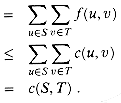
The FORD-FULKERSON algorithm simply expands on the FORD-FULKER-SON-METHOD pseudocode given earlier. Figure 27.6 shows the result of each iteration in a sample run. Lines 1-3 initialize the flow â to 0. The while loop of lines 4-8 repeatedly finds an augmenting path p in Gâ and augments flow â along p by the residual capacity câ(p). When no augmenting paths exist, the flow â is a maximum flow.
The running time of FORD-FULKERSON depends on how the augmenting path p in line 4 is determined. If it is chosen poorly, the algorithm might not even terminate: the value of the flow will increase with successive augmentations, but it need not even converge to the maximum flow value. If the augmenting path is chosen by using a breadth-first search (Section 23.2), however, the algorithm runs in polynomial time. Before proving this, however, we obtain a simple bound for the case in which the augmenting path is chosen arbitrarily and all capacities are integers.
Most often in practice, the maximum-flow problem arises with integral capacities. If the capacities are rational numbers, an appropriate scaling transformation can be used to make them all integral. Under this assumption, a straightforward implementation of FORD-FULKERSON runs in time O(E | â* |), where â* is the maximum flow found by the algorithm. The analysis is as follows. Lines 1-3 take time
The work done within the while loop can be made efficient if we efficiently manage the data structure used to implement the network G = (V, E). Let us assume that we keep a data structure corresponding to a directed graph G' = (V, E'), where E' = {(u, v) : (u, v)
When the capacities are integral and the optimal flow value | â* | is small, the running time of the Ford-Fulkerson algorithm is good. Figure 27.7(a) shows an example of what can happen on a simple flow network for which | â* | is large. A maximum flow in this network has value 2,000,000: 1,000,000 units of flow traverse the path s
The bound on FORD-FULKERSON can be improved if we implement the computation of the augmenting path p in line 4 with a breadth-first search, that is, if the augmenting path is a shortest path from s to t in the residual network, where each edge has unit distance (weight). We call the Ford-Fulkerson method so implemented the Edmonds-Karp algorithm. We now prove that the Edmonds-Karp algorithm runs in O(V E2) time.
The analysis depends on the distances to vertices in the residual network Gf. The following lemma uses the notation
Lemma 27.8
If the Edmonds-Karp algorithm is run on a flow network G = (V, E) with source s and sink t, then for all vertices v
Proof Suppose for the purpose of contradiction that for some vertex v
We can assume without loss of generality that
We now take a shortest path p' in G
With vertices v and u thus established, we can consider the net flow â from u to v before the augmentation of flow in G
which contradicts our assumption that the flow augmentation decreases the distance from s to v.
Thus, we must have
which contradicts our initial assumption.
The next theorem bounds the number of iterations of the Edmonds-Karp algorithm.
Theorem 27.9
If the Edmonds-Karp algorithm is run on a flow network G = (V, E) with source s and sink t, then the total number of flow augmentations performed by the algorithm is at most O(V E).
Proof We say that an edge (u, v) in a residual network G
Let u and v be vertices in V that are connected by an edge in E. How many times can (u, v) be a critical edge during the execution of the Edmonds-Karp algorithm? Since augmenting paths are shortest paths, when (u, v) is critical for the first time, we have
Once the flow is augmented, the edge (u, v) disappears from the residual network. It cannot reappear later on another augmenting path until after the net flow from u to v is decreased, and this only happens if (v, u) appears on an augmenting path. If
Since
Consequently, from the time (u, v) becomes critical to the time when it next becomes critical, the distance of u from the source increases by at least 2. The distance of u from the source is initially at least 1, and until it becomes unreachable from the source, if ever, its distance is at most
Since each iteration of FORD-FULKERSON can be implemented in O(E) time when the augmenting path is found by breadth-first search, the total running time of the Edmonds-Karp algorithm is O(V E2). The algorithm of Section 27.4 gives a method for achieving an O(V2 E) running time, which forms the basis for the O(V3)-time algorithm of Section 27.5.
27.2-1
In Figure 27.1(b), what is the flow across the cut ({s, v2, v4} , {v1, v3, t})? What is the capacity of this cut?
27.2-2
Show the execution of the Edmonds-Karp algorithm on the flow network of Figure 27.1(a).
27.2-3
In the example of Figure 27.6, what is the minimum cut corresponding to the maximum flow shown? Of the augmenting paths appearing in the example, which two cancel flow that was previously shipped?
27.2-4
Prove that for any pair of vertices u and v and any capacity and flow functions c and f, we have c
27.2-5
Recall that the construction in Section 27.1 that converts a multisource, multisink flow network into a single-source, single-sink network adds edges with infinite capacity. Prove that any flow in the resulting network has a finite value if the edges of the original multisource, multisink network have finite capacity.
27.2-6
Suppose that each source si in a multisource, multisink problem produces exactly pi units of flow, so that
27.2-7
Prove Lemma 27.3.
27.2-8
Show that a maximum flow in a network G = (V, E) can always be found by a sequence of at most |E| augmenting paths. (Hint: Determine the paths after finding the maximum flow.)
27.2-9
The edge connectivity of an undirected graph is the minimum number k of edge that must be removed to disconnect the graph. For example, the edge connectivity of a tree is 1, and the edge connectivity of a cyclic chain of vertices is 2. Show how the edge connectivity of an undirected graph G = (V, E) can be determined by running a maximum-flow algorithm on at most |V| flow network, each having O(V) vertices and O(E) edges.
27.2-10
Show that the Edmonds-Karp algorithm terminates after at most |V| |E| /4 iterations. (Hint: For any edge (u, v), consider how both
Some combinatorial problems can easily be cast as maximum-flow problems. The multiple-source, multiple-sink maximum-flow problem from Section 27.1 gave us one example. There are other combinatorial problems that seem on the surface to have little to do with flow networks, but can in fact be reduced to a maximum-flow problem. This section presents one such problem: finding a maximum matching in a bipartite graph (see Section 5.4). In order to solve this problem, we shall take advantage of an integrality property provided by the Ford-Fulkerson method. We shall also see that the Ford-Fulkerson method can be made to solve the maximum-bipartite-matching problem on a graph G = (V, E) in O(V E) time.
Given an undirected graph G = (V, E), a matching is a subset of edges M
The problem of finding a maximum matching in a bipartite graph has many practical applications. As an example, we might consider matching a set L of machines with a set R of tasks to be performed simultaneously. We take the presence of edge (u, v) in E to mean that a particular machine u
We can use the Ford-Fulkerson method to find a maximum matching in an undirected bipartite graph G = (V, E) in time polynomial in |V| and |E|. The trick is to construct a flow network in which flows correspond to matchings, as shown in Figure 27.9. We define the corresponding flow network G' = (V', E') for the bipartite graph G as follows. We let the sources s and sink t be new vertices not in V, and we let V'= V
To complete the construction, we assign unit capacity to each edge in E'.
The following theorem shows that a maching in G corresponds directly to a flow in G's corresponding flow network G'. We say that a flow
Lemma 27.10
Let G = (V, E) be a bipartite graph with vertex partition V = L
Proof We first show that a matching M in G corresponds to an integer-valued flow in G'. Define f as follows. If (u, v)
Intuitively, each edge (u, v)
To prove the converse, let f be an integer-valued flow in G' and let
Each vertex u
To see that |M| = |f|, observe that for every matched vertex u
It is intuitive that a maximum matching in a bipartite graph G corresponds to a maximum flow in its corresponding flow network G'. Thus, we can compute a maximum matching in G by running a maximum-flow algorithm on G'. The only hitch in this reasoning is that the maximum-flow algorithm might return a flow in G' that consists of nonintegral amounts. The following theorem shows that if we use the Ford-Fulkerson method, this difficulty cannot arise.
Theorem 27.11
If the capacity function c takes on only integral values, then the maximum flow â produced by the Ford-Fulkerson method has the property that |â| is integer-valued. Moreover, for all vertices u and v, the value of â(u, v) is an integer.
Proof The proof is by induction on the number of iterations. We leave it as Exercise 27.3-2.
We can now prove the following corollary to Lemma 27.10.
Corollary 27.12
The cardinality of a maximum matching in a bipartite graph G is the value of a maximum flow in its corresponding flow network G'.
Proof We use the nomenclature from Lemma 27.10. Suppose that M is a maximum matching in G and that the corresponding flow f in G' is not maximum. Then there is a maximum flow f' in G' such that |f'| > |f|. Since the capacities in G' are integer-valued, by Theorem 27.11, so is f'. Thus, f' corresponds to a matching M' in G with cardinality |M'| = |f'| > |f| = |M|, contradicting the maximality of M. In a similar manner, we can show that if f is a maximum flow in G', its corresponding matching is a maximum matching on G.
Thus, given a bipartite undirected graph G, we can find a maximum matching by creating the flow network G', running the Ford-Fulkerson method, and directly obtaining a maximum matching M from the integer-valued maximum flow f found. Since any matching in a bipartite graph has cardinality at most min(L, R) = O(V), the value of the maximum flow in G' is O(V). We can therefore find a maximum matching in a bipartite graph in time O(V E).
27.3-1
Run the Ford-Fulkerson algorithm on the flow network in Figure 27.9(b) and show the residual network after each flow augmentation. Number the vertices in L top to bottom from 1 to 5 and in R top to bottom from 6 to 9. For each iteration, pick the augmenting path that is lexicographically smallest.
27.3-2
Prove Theorem 27.11.
27.3-3
Let G = (V, E) be a bipartite graph with vertex partition V = L
27.3-4
A perfect matching is a matching in which every vertex is matched. Let G = (V, E) be an undirected bipartite graph with vertex partition V = L
that is, the set of vertices adjacent to some member of X. Prove Hall's theorem: there exists a perfect matching in G if and only if |A|
27.3-5
A bipartite graph G = (V, E), where V = L
In this section, we present the "preflow-push" approach to computing maximum flows. The fastest maximum-flow algorithms to date are preflow-push algorithms, and other flow problems, such as the minimum-cost flow problem, can be solved efficiently by preflow-push methods. This section introduces Goldberg's "generic" maximum-flow algorithm, which has a simple implementation that runs in O(V2 E) time, thereby improving upon the O(V E2) bound of the Edmonds-Karp algorithm. Section 27.5 refines the generic algorithm to obtain another preflow-push algorithm that runs in O(V3) time.
Preflow-push algorithms work in a more localized manner than the Ford-Fulkerson method. Rather than examine the entire residual network G = (V, E) to find an augmenting path, preflow-push algorithms work on one vertex at a time, looking only at the vertex's neighbors in the residual network. Furthermore, unlike the Ford-Fulkerson method, preflow-push algorithms do not maintain the flow-conservation property throughout their execution. They do, however, maintain a preflow, which is a function f : V X V
We say that a vertex u
We shall start this section by describing the intuition behind the preflow-push method. We shall then investigate the two operations employed by the method: "pushing" preflow and "lifting" a vertex. Finally, we shall present a generic preflow-push algorithm and analyze its correctness and running time.
The intuition behind the preflow-push method is probably best understood in terms of fluid flows: we consider a flow network G = (V, E) to be a system of interconnected pipes of given capacities. Applying this analogy to the Ford-Fulkerson method, we might say that each augmenting path in the network gives rise to an additional stream of fluid, with no branch points, flowing from the source to the sink. The Ford-Fulkerson method iteratively adds more streams of flow until no more can be added.
The generic preflow-push algorithm has a somewhat different intuition. As before, directed edges correspond to pipes. Vertices, which are pipe junctions, have two interesting properties. First, to accommodate excess flow, each vertex has an outflow pipe leading to an arbitrarily large reservoir that can accumulate fluid. Second, each vertex, its reservoir, and all its pipe connections are on a platform whose height increases as the algorithm progresses.
Vertex heights determine how flow is pushed: we only push flow downhill, that is, from a higher vertex to a lower vertex. There may be positive net flow from a lower vertex to a higher vertex, but operations that push flow always push it downhill. The height of the source is fixed at |V|, and the height of the sink is fixed at 0. All other vertex heights start at 0 and increase with time. The algorithm first sends as much flow as possible downhill from the source toward the sink. The amount it sends is exactly enough to fill each outgoing pipe from the source to capacity; that is, it sends the capacity of the cut (s, V - s). When flow first enters an intermediate vertex, it collects in the vertex's reservoir. From there, it is eventually pushed downhill.
It may eventually happen that the only pipes that leave a vertex u and are not already saturated with flow connect to vertices that are on the same level as u or are uphill from u. In this case, to rid an overflowing vertex u of its excess flow, we must increase its height--an operation called "lifting" vertex u. Its height is increased to one unit more than the height of the lowest of its neighbors to which it has an unsaturated pipe. After a vertex is lifted, therefore, there is at least one outgoing pipe through which more flow can be pushed.
Eventually, all the flow that can possibly get through to the sink has arrived there. No more can arrive, because the pipes obey the capacity constraints; the amount of flow across any cut is still limited by the capacity of the cut. To make the preflow a "legal" flow, the algorithm then sends the excess collected in the reservoirs of overflowing vertices back to the source by continuing to lift vertices to above the fixed height |V| of the source. (Shipping the excess back to the source is actually accomplished by canceling the flows that cause the excess.) As we shall see, once all the reservoirs have been emptied, the preflow is not only a "legal" flow, it is also a maximum flow.
From the preceding discussion, we see that there are two basic operations performed by a preflow-push algorithm: pushing flow excess from a vertex to one of its neighbors and lifting a vertex. The applicability of these operations depends on the heights of vertices, which we now define precisely.
Let G = (V, E) be a flow network with source s and sink t, and let f be a preflow in G. A function h: V
for every residual edge (u, v)
Lemma 27.13
Let G = (V, E) be a flow network, let f be a preflow in G, and let h be a height function on V. For any two vertices u, v
The basic operation PUSH(u, v) can be applied if u is an overflowing vertex, cf (u, v) > 0, and h(u) = h(v) + 1. The pseudocode below updates the preflow f in an implied network G = (V, E). It assumes that the capacities are given by a constant-time function c and that residual capacities can also be computed in constant time given c and f . The excess flow stored at a vertex u is maintained as e[u], and the height of u is maintained as h[u]. The expression df(u, v) is a temporary variable that stores the amount of flow that can be pushed from u to v.
The code for PUSH operates as follows. Vertex u is assumed to have a positive excess e[u], and the residual capacity of (u, v) is positive. Thus, we can ship up to df(u, v) = min (e[u], cf(u, v)) units of flow from u to v without causing e[u] to become negative or the capacity c(u, v) to be exceeded. This value is computed in line 3. We move the flow from u to v by updating f in lines 4-5 and e in lines 6-7. Thus, if â is a preflow before PUSH is called, it remains a preflow afterward.
Observe that nothing in the code for PUSH depends on the heights of u and v, yet we prohibit it from being invoked unless h[u] = h[v] + 1. Thus, excess flow is only pushed downhill by a height differential of 1. By Lemma 27.13, no residual edges exist between two vertices whose heights differ by more than 1, and thus there is nothing to be gained by allowing flow to be pushed downhill by a height differential of more than 1.
We call the operation PUSH(u, v) a push from u to v. If a push operation applies to some edge (u, v) leaving a vertex u, we also say that the push operation applies to u. It is a saturating push if edge (u, v) becomes saturated (cf (u, v) = 0 afterward); otherwise, it is a nonsaturating push. If an edge is saturated, it does not appear in the residual network.
The basic operation LIFT(u) applies if u is overflowing and if cf (u, v) > 0 implies h[u]
When we call the operation LIFT(u), we say that vertex u is lifted. It is important to note that when u is lifted, Ef must contain at least one edge that leaves u, so that the minimization in the code is over a nonempty set. This fact follows from the assumption that u is overflowing. Since e[u] > 0, we have e[u] = f [V, u] > 0, and hence there must be at least one vertex v such that â[v, u] > 0. But then,
which implies that (u, v)
The generic preflow-push algorithm uses the following subroutine to create an initial preflow in the flow network.
That is, each edge leaving the source is filled to capacity, and all other edges carry no flow. For each vertex v adjacent to the source, we initially have e[v] = c(s, v). The generic algorithm also begins with an initial height function h, given by
This is a height function because the only edges (u, v) for which h[u] > h[v] + 1 are those for which u = s, and those edges are saturated, which means that they are not in the residual network.
The following algorithm typifies the preflow-push method.
After initializing the flow, the generic algorithm repeatedly applies, in any order, the basic operations wherever they are applicable. The following lemma tells us that as long as an overflowing vertex exists, at least one of the two operations applies.
Lemma 27.14
Let G = (V, E) be a flow network with source s and sink t, let
Proof For any residual edge (u, v), we have h(u)
To show that the generic preflow-push algorithm solves the maximum-flow problem, we shall first prove that if it terminates, the preflow
Lemma 27.15
During the execution of GENERIC-PREFLOW-PUSH on a flow network G = (V, E), for each vertex u
Proof Because vertex heights change only during lift operations, it suffices to prove the second statement of the lemma. If vertex u is lifted, then for all vertices v such that (u, v)
Lemma 27.16
Let G = (V, E) be a flow network with source s and sink t. During the execution of GENERIC-PREFLOW-PUSH on G, the attribute h is maintained as a height function.
Proof The proof is by induction on the number of basic operations performed. Initially, h is a height function, as we have already observed.
We claim that if h is a height function, then an operation LIFT(u) leaves h a height function. If we look at a residual edge (u, v)
Now, consider an operation PUSH(u, v). This operation may add the edge (v, u) to E
The following lemma gives an important property of height functions.
Lemma 27.17
Let G = (V, E) be a flow network with source s and sink t, let f be a preflow in G, and let h be a height function on V. Then, there is no path from the source s to the sink t in the residual network G
Proof Assume for the sake of contradiction that there is a path p =
We are now ready to show that if the generic preflow-push algorithm terminates, the preflow it computes is a maximum flow.
Theorem 27.18
If the algorithm GENERIC-PREFLOW-PUSH terminates when run on a flow network G = (V, E) with source s and sink t, then the preflow f it computes is a maximum flow for G.
Proof If the generic algorithm terminates, then each vertex in V - {s, t} must have an excess of 0, because by Lemmas 27.14 and 27.16 and the invariant that
To show that the generic preflow-push algorithm indeed terminates, we shall bound the number of operations it performs. Each of the three types of operations--lifts, saturating pushes, and nonsaturating pushes--is bounded separately. With knowledge of these bounds, it is a straightforward problem to construct an algorithm that runs in O(V2 E) time. Before beginning the analysis, however, we prove an important lemma.
Lemma 27.19
Let G = (V, E) be a flow network with source s and sink t, and let
Proof Let U = {v: there exists a simple path from u to v in G
We claim for each pair of vertices v
Thus, we must have
Excesses are nonnegative for all vertices in V - {s}; because we have assumed that U
The next lemma bounds the heights of vertices, and its corollary bounds the number of lift operations that are performed in total.
Lemma 27.20
Let G = (V, E) be a flow network with source s and sink t. At any time during the execution of GENERIC-PREFLOW-PUSH on G, we have h[u]
Proof The heights of the source s and the sink t never change because these vertices are by definition not overflowing. Thus, we always have h[s] = |V| and h[t] = 0.
Because a vertex is lifted only when it is overflowing, we can consider any overflowing vertex u
Corollary 27.21
Let G = (V, E) be a flow network with source s and sink t. Then, during the execution of GENERIC-PREFLOW-PUSH on G, the number of lift operations is at most 2 |V| - 1 per vertex and at most (2 |V| - 1)(|V| - 2) < 2 |V |2 overall.
Proof Only vertices in V - {s, t}, which number |V| - 2, may be lifted. Let u
Lemma 27.20 also helps us to bound the number of saturating pushes.
Lemma 27.22
During the execution of GENERIC-PREFLOW-PUSH on any flow network G = (V, E), the number of saturating pushes is at most 2 |V| |E|.
Proof For any pair of vertices u, v
Consider the sequence A of integers given by h[u] + h[v] for each saturating push that occurs between vertices u and v. We wish to bound the length of this sequence. When the first push in either direction between u and v occurs, we must have h[u] + h[v]
The following lemma bounds the number of nonsaturating pushes in the generic preflow-push algorithm.
Lemma 27.23
During the execution of GENERIC-PREFLOW-PUSH on any flow network G = (V, E), the number of nonsaturating pushes is at most 4
Proof Define a potential function
Thus, during the course of the algorithm, the total amount of increase in
We have now set the stage for the following analysis of the GENERIC-PREFLOW-PUSH procedure, and hence of any algorithm based on the preflow-push method.
Theorem 27.24
During the execution of GENERIC-PREFLOW-PUSH on any flow network G = (V, E), the number of basic operations is O(V2 E).
Proof Immediate from Corollary 27.21 and Lemmas 27.22 and 27.23.
Corollary 27.25
There is an implementation of the generic preflow-push algorithm that runs in O(V2 E) time on any flow network G = (V, E).
Proof Exercise 27.4-1 asks you to show how to implement the generic algorithm with an overhead of O(V) per lift operation and O(1) per push. The corollary then follows.
27.4-1
Show how to implement the generic preflow-push algorithm using O(V) time per lift operation and O(1) time per push, for a total time of O(V2 E).
27.4-2
Prove that the generic preflow-push algorithm spends a total of only O(V E) time in performing all the O(V2) lift operations.
27.4-3
Suppose that a maximum flow has been found in a flow network G = (V, E) using a preflow-push algorithm. Give a fast algorithm to find a minimum cut in G.
27.4-4
Give an efficient preflow-push algorithm to find a maximum matching in a bipartite graph. Analyze your algorithm.
27.4-5
Suppose that all edge capacities in a flow network G = (V, E) are in the set {1, 2, . . . , k}. Analyze the running time of the generic preflow-push algorithm in terms of
27.4-6
Show that line 7 of INITIALIZE-PREFLOW can be changed to
without affecting the correctness or asymptotic performance of the generic preflow-push algorithm.
27.4-7
Let
27.4-8
As in the previous exercise, let
27.4-9
Show that the number of nonsaturating pushes executed by GENERIC-PREFLOW-PUSH on a flow network G = (V, E) is at most 4
The preflow-push method allows us to apply the basic operations in any order at all. By choosing the order carefully and managing the network data structure efficiently, however, we can solve the maximum-flow problem faster than the O(V2E) bound given by Corollary 27.25. We shall now examine the lift-to-front algorithm, a preflow-push algorithm whose running time is O(V3), which is asymptotically at least as good as O(V2E).
The lift-to-front algorithm maintains a list of the vertices in the network. Beginning at the front, the algorithm scans the list, repeatedly selecting an overflowing vertex u and then "discharging" it, that is, performing push and lift operations until u no longer has a positive excess. Whenever a vertex is lifted, it is moved to the front of the list (hence the name "lift-to-front") and the algorithm begins its scan anew.
The correctness and analysis of the lift-to-front algorithm depend on the notion of "admissible" edges: those edges in the residual network through which flow can be pushed. After proving some properties about the network of admissible edges, we shall investigate the discharge operation and then present and analyze the lift-to-front algorithm itself.
If G = (V, E) is a flow network with source s and sink t,
The admissible network consists of those edges through which flow can be pushed. The following lemma shows that this network is a directed acyclic graph (dag).
Lemma 27.26
If G = (V,E) is a flow network,
Proof The proof is by contradiction. Suppose that G
Because each vertex in cycle p appears once in each of the summations, we derive the contradiction that 0 = k.
The next two lemmas show how push and lift operations change the admissible network.
Lemma 27.27
Let G = (V,E) be a flow network, let
Proof By the definition of an admissible edge, flow can be pushed from u to v. Since u is overflowing, the operation PUSH(u, v) applies. The only new residual edge that can be created by pushing flow from u to v is the edge (v, u). Since h(v) = h(u) - 1, edge (v, u) cannot become admissible. If the operation is a saturating push, then c
Lemma 27.28
Let G = (V,E) be a flow network, let
Proof If u is overflowing, then by Lemma 27.14, either a push or a lift operation applies to it. If there are no admissible edges leaving u, no flow can be pushed from u and LIFT(u) applies. After the lift operation, h[u] = 1 + min {h[v]: (u,v)
To show that no admissible edges enter u after a lift operation, suppose that there is a vertex v such that (v,u) is admissible. Then, h[
Edges in the lift-to-front algorithm are organized into "neighbor lists." Given a flow network G = (V,E), the neighbor list N[u] for a vertex u
The lift-to-front algorithm cycles through each neighbor list in an arbitrary order that is fixed throughout the execution of the algorithm. For each vertex u, the field current[u] points to the vertex currently under consideration in N[u]. Initially, current[u] is set to head[N[u]].
An overflowing vertex u is discharged by pushing all of its excess flow through admissible edges to neighboring vertices, lifting u as necessary to cause edges leaving u to become admissible. The pseudocode goes as follows.
Figure 27.10 steps through several iterations of the while loop of lines 1-8, which executes as long as vertex u has positive excess. Each iteration performs exactly one of three actions, depending on the current vertex
1. If v is NIL, then we have run off the end of N[u]. Line 4 lifts vertex u, and then line 5 resets the current neighbor of u to be the first one in N[u]. (Lemma 27.29 below states that the lift operation applies in this situation.)
2. If v is non-NIL and (u, v) is an admissible edge (determined by the test in line 6), then line 7 pushes some (or possibly all) of u's excess to vertex
3. If v is non-NIL but (u, v) is inadmissible, then line 8 advances current[u] one position further in the neighbor list N[u].
Observe that if DISCHARGE is called on an overflowing vertex u, then the last action performed by DISCHARGE must be a push from u. Why? The procedure terminates only when e[u] becomes zero, and neither the lift operation nor the advancing of the pointer current[u] affects the value of e[u].
We must be sure that when PUSH or LIFT is called by DISCHARGE, the operation applies. The next lemma proves this fact.
Lemma 27.29
If DISCHARGE calls PUSH(u, v) in line 7, then a push operation applies to (u, v). If DISCHARGE calls LIFT(u) in line 4, then a lift operation applies to u.
Proof The tests in lines 1 and 6 ensure that a push operation occurs only if the operation applies, which proves the first statement in the lemma.
To prove the second statement, according to the test in line 1 and Lemma 27.28, we need only show that all edges leaving u are inadmissible. Observe that as DISCHARGE(u) is repeatedly called, the pointer current[u] moves down the list N[u]. Each "pass" begins at the head of N[u] and finishes with current[u] = NIL, at which point u is lifted and a new pass begins. For the current[u] pointer to advance past a vertex
In the lift-to-front algorithm, we maintain a linked list L consisting of all vertices in V - {s, t}. A key property is that the vertices in L are topologically sorted according to the admissible network. (Recall from Lemma 27.26 that the admissible network is a dag.)
The pseudocode for the lift-to-front algorithm assumes that the neighbor lists N[u] have already been created for each vertex u. It also assumes that next[u] points to the vertex that follows u in list L and that, as usual, next[u] = NIL if u is the last vertex in the list.
The lift-to-front algorithm works as follows. Line 1 initializes the preflow and heights to the same values as in the generic preflow-push algorithm. Line 2 initializes the list L to contain all potentially overflowing vertices, in any order. Lines 3-4 initialize the current pointer of each vertex u to the first vertex in u's neighbor list.
As shown in Figure 27.11, the while loop of lines 6-11 runs through the list L, discharging vertices. Line 5 makes it start with the first vertex in the list. Each time through the loop, a vertex u is discharged in line 8. If u was lifted by the DISCHARGE procedure, line 10 moves it to the front of list L. This determination is made by saving u's height in the variable old-height before the discharge operation (line 7) and comparing this saved height to u's height afterward (line 9). Line 11 makes the next iteration of the while loop use the vertex following u in list L. If u was moved to the front of the list, the vertex used in the next iteration is the one following u in its new position in the list.
To show that LIFT-TO-FRONT computes a maximum flow, we shall show that it is an implementation of the generic preflow-push algorithm. First, observe that it only performs push and lift operation when they apply, since Lemma 27.29 guarantees that DISCHARGE only performs them when they apply. It remains to show that when LIFT-TO-FRONT terminates, no basic operations apply. Observe that if u reaches the end of L, every vertex in L must have been discharged without causing a lift. Lemma 27.30, which we shall prove in a moment, states that the list L is maintained as a topological sort of the admissible network. Thus, a push operation causes excess flow to move to vertices further down the list (or to s or t). If the pointer u reaches the end of the list, therefore, the excess of every vertex is 0, and no basic operations apply.
Lemma 27.30
If we run LIFT-TO-FRONT on a flow network G = (V, E) with source s and sink t, then each iteration of the while loop in lines 6-11 maintains the invariant that list L is a topological sort of the vertices in the admissible network G
Proof Immediately after INITIALIZE-PREFLOW has been run, h[s] =
We now show that the invariant is maintained by each iteration of the while loop. The admissible network is changed only by push and lift operations. By Lemma 27.27, push operations only make edges inadmissible. Thus, admissible edges can be created only by lift operations. After a vertex is lifted, however, Lemma 27.28 states that there are no admissible edges entering u but there may be admissible edges leaving u. Thus, by moving u to the front of L, the algorithm ensures that any admissible edges leaving u satisfy the topological sort ordering.
We shall now show that LIFT-TO-FRONT runs in O(V3) time on any flow network G = (V, E). Since the algorithm is an implementation of the generic preflow-push algorithm, we shall take advantage of Corollary 27.21, which provides an O(V) bound on the number of lift operations executed per vertex and an O(V2) bound on the total number of lifts overall. In addition, Exercise 27.4-2 provides an O(V E) bound on the total time spent performing lift operations, and Lemma 27.22 provides an O(V E) bound on the total number of saturating push operations.
Theorem 27.31
The running time of LIFT-TO-FRONT on any flow network G = (V, E) is O(V3).
Proof Let us consider a "phase" of the lift-to-front algorithm to be the time between two consecutive lift operations. There are O(V2) phases, since there are O(V2) lift operations. Each phase consists of at most |V | calls to DISCHARGE, which can be seen as follows. If DISCHARGE does not perform a lift operation, the next call to DISCHARGE is further down the list L, and the length of L is less than |V |. If DISCHARGE does perform a lift, the next call to DISCHARGE belongs to a different phase. Since each phase contains at most |V | calls to DISCHARGE and there are O(V2) phases, the number of times DISCHARGE is called in line 8 of LIFT-TO-FRONT is O(V3). Thus, the total work performed by the while loop in LIFT-TO-FRONT, excluding the work performed within DISCHARGE, is at most O(V3).
We must now bound the work performed within DISCHARGE during the execution of the algorithm. Each iteration of the while loop within DISCHARGE performs one of three actions. We shall analyze the total amount of work involved in performing each of these actions.
We start with lift operations (lines 4-5). Exercise 27.4-2 provides an O(V E) time bound on all the O(V2) lifts that are performed.
Now, suppose that the action updates the current[u] pointer in line 8. This action occurs O(degree(u)) times each time a vertex u is lifted, and O(V
The third type of action performed by DISCHARGE is a push operation (line 7). We already know that the total number of saturating push operations is O(V E). Observe that if a nonsaturating push is executed, DISCHARGE immediately returns, since the push reduces the excess to 0. Thus, there can be at most one nonsaturating push per call to DISCHARGE. As we have observed, DISCHARGE is called O(V3) times, and thus the total time spent performing nonsaturating pushes is O(V3).
The running time of LIFT-TO-FRONT is therefore O(V3 + V E), which is O(V3).
27.5-1
Illustrate the execution of LIFT-TO-FRONT in the manner of Figure 27.11 for the flow network in Figure 27.1 (a). Assume that the initial ordering of vertices in L is
27.5-2
We would like to implement a preflow-push algorithm in which we maintain a first-in, first-out queue of overflowing vertices. The algorithm repeatedly discharges the vertex at the head of the queue, and any vertices that were not overflowing before the discharge but are overflowing afterward are placed at the end of the queue. After the vertex at the head of the queue is discharged, it is removed. When the queue is empty, the algorithm terminates. Show that this algorithm can be implemented to compute a maximum flow in O(V3) time.
27.5-3
Show that the generic algorithm still works if LIFT updates h[u] by simply computing h[u]
27.5-4
Show that if we always discharge a highest overflowing vertex, the preflow-push method can be made to run in O(V3) time.
27-1 Escape problem
An n x n grid is an undirected graph consisting of n rows and n columns of vertices, as shown in Figure 27.12. We denote the vertex in the ith row and the jth column by (i, j). All vertices in a grid have exactly four neighbors, except for the boundary vertices, which are the points (i, j) for which i = 1, i = n, j = 1, or j = n.
Given m
a. Consider a flow network in which vertices, as well as edges, have capacities. That is, the positive net flow entering any given vertex is subject to a capacity constraint. Show that determining the maximum flow in a network with edge and vertex capacities can be reduced to an ordinary maximum-flow problem on a flow network of comparable size.
b. Describe an efficient algorithm to solve the escape problem, and analyze its running time.
27-2 Minimum path cover
A path cover of a directed graph G = (V, E) is a set P of vertex-disjoint paths such that every vertex in V is included in exactly one path in P. Paths may start and end anywhere, and they may be of any length, including 0. A minimum path cover of G is a path cover containing the fewest possible paths.
a. Give an efficient algorithm to find a minimum path cover of a directed acyclic graph G = (V, E). (Hint: Assuming that V = {1, 2, . . . , n}, construct the graph G' = (V', E'), where
b. Does your algorithm work for directed graphs that contain cycles? Explain.
27-3 Space shuttle experiments
Professor Spock is consulting for NASA, which is planning a series of space shuttle flights and must decide which commercial experiments to perform and which instruments to have on board each flight. For each flight, NASA considers a set E = {E1, E2, . . . , Em} of experiments, and the commercial sponsor of experiment Ej has agreed to pay NASA pj dollars for the results of the experiment. The experiments use a set I = {I1, I2, . . . , In} of instruments; each experiment Ej requires all the instruments in a subset Rj
Consider the following network G. The network contains a source vertex s, vertices I1, I2, . . . , In, vertices E1, E2, . . . , Em, and a sink vertex t. For k = 1, 2 . . . , n, there is an edge (s, Ik) of capacity ck, and for j = 1, 2, . . . , m, there is an edge (Ej, t) of capacity pj. For k = 1, 2, . . . , n and j = 1, 2, . . . , m, if Ik
a. Show that if Ej
b. Show how to determine the maximum net revenue from the capacity of the minimum cut of G and the given pj values.
c. Give an efficient algorithm to determine which experiments to perform and which instruments to carry. Analyze the running time of your algorithm in terms of m, n, and 27.1 Flow networks
Flow networks and flows
 E has a nonnegative capacity c(u, v)
  0. If (u, v)
  E, we assume that c(u, v) = 0. We distinguish two vertices in a flow network: a source s and a sink t. For convenience, we assume that every vertex lies on some path from the source to the sink. That is, for every vertex v V, there is a path
  . The graph is therefore connected, and |E| |V| - 1. Figure 27.1 shows an example of a flow network.
 R that satisfies the following three properties: V, we require â (u, v)
  c(u, v). V, we require â (u, v) = -â (v, u). V - {s, t}, we require
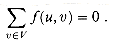
(27.1)
 | notation denotes flow value, not absolute value or cardinality.) In the maximum-flow problem, we are given a flow network G with source s and sink t, and we wish to find a flow of maximum value from s to t. V, we have â (u, u) = - f (u,u), which implies that â (u, u) = 0. The flow-conservation property says that the total net flow out of a vertex other than the source or sink is 0. By skew symmetry, we can rewrite the flow-conservation property as
 V - {s, t}. That is, the total net flow into a vertex is 0.
Figure 27.1 (a) A flow network G = (V, E) for the Lucky Puck Company's trucking problem. The Vancouver factory is the source s, and the Winnipeg warehouse is the sink t. Pucks are shipped through intermediate cities, but only c (u, v) crates per day can go from city u to city v. Each edge is labeled with its capacity. (b) A flow â in G with value |â| = 19. Only positive net flows are shown. If â (u, v) > 0, edge (u, v) is labeled by â (u, v)/c(u, v). (The slash notation is used merely to separate the flow and capacity; it does not indicate division.) If â (u,v)
0, edge (u, v) is labeled only by its capacity. E nor (v, u) E, then c(u, v) = c(v, u) = 0. Hence, by the capacity constraint, â(u, v) 0 and â (v, u) 0. But since â (u, v) = - â (v, u), by skew symmetry, we have â(u, v) = â(v, u) = 0. Thus, nonzero net flow from vertex u to vertex v implies that (u, v) E or (v, u) E (or both).
(27.2)
An example of network flow
Figure 27.2 Cancellation. (a) Vertices v1, and v2, with c(v1, v2) = 10 and c(v2, v1 ) = 4. (b) How we indicate the net flow when 8 crates per day are shipped from v1 to v2. (c) An additional shipment of 3 crates per day is made from v2 to v1. (d) By cancelling flow going in opposite directions, we can represent the situation in (c) with positive net flow in one direction only. (e) Another 7 crates per day is shipped from v2 to v1.
Figure 27.3 Converting a multiple-source, multiple-sink maximum-flow problem into a problem with a single source and a single sink. (a) A flow network with five sources S = {s1, s2, s3, s4, s5} and three sinks T={t1, t2, t3}. (b) An equivalent single-source, single-sink flow network. We add a supersource s' and an edge with infinite capacity from s' to each of the multiple sources. We also add a supersink t' and an edge with infinite capacity from each of the multiple sinks to t'.
Networks with multiple sources and sinks
 for each i = 1, 2, . . . , m. We also create a new supersink t and add a directed edge (tj, t) with capacity c(tj, t) = for each i = 1, 2, . . . , n. Intuitively, any flow in the network in (a) corresponds to a flow in the network in (b), and vice versa. The single source s simply provides as much flow as desired for the multiple sources si, and the single sink t likewise consumes as much flow as desired for the multiple sinks ti. Exercise 27.1-3 asks you to prove formally that the two problems are equivalent.
Working with flows
 V -{s, t}. Also, for convenience, we shall typically omit set braces when they would otherwise be used in the implicit summation notation. For example, in the equation f(s, V - s) = f(s, V), the term V - s means the set V - {s}.
 V ,
V ,f(X, X) = 0 .
V ,f(X, Y) = -f(Y, X) .
V with  ,
,f(X
 Y, Z) = f(X, Z) + f(Y, Z)
f(Z, X
Y) = f(Z, X) + f(Z, Y) . |f| = f(V, t) .
(27.3)
|f| = f(s, V) (by definition)
= f(V, V) - f(V - s, V) (by Lemma 27.1)
= f(V, V - s) (by Lemma 27.1)
= f(V, t) + f(V, V - s - t) (by Lemma 27.1 )
= f(V, t) (by flow conservation) .
Exercises
V for which f(X, Y) = -f(V - X, Y). Then, find a pair of subsets X, Y V for which f(X, Y)  - f(V - X, Y).
(f1 + f2)(u, v) = f1(u, v) + f2(u, v)
(27.4)
V. If f1 and f2 are flows in G, which of the three flow properties must the flow sum f1 + f2 satisfy, and which might it violate? be a real number. The scalar flow product f is a function from V X V to R defined by
(
f)(u, v) = f(u, v).f1 + (1 - ) f2 for all in the range 0 1.27.2 The Ford-Fulkerson method
V, giving an initial flow of value 0. At each iteration, we increase the flow value by finding an "augmenting path," which we can think of simply as a path from the source s to the sink t along which we can push more flow, and then augmenting the flow along this path. We repeat this process until no augmenting path can be found. The max-flow min-cut theorem will show that upon termination, this process yields a maximum flow.FORD-FULKERSON-METHOD(G, s, t)
1 initialize flow f to 0
2 while there exists an augmenting path p
3 do augment flow f along p
4 return f
Residual networks
V. The amount of additional net flow we can push from u to v before exceeding the capacity c(u, v) is the residual capacity of (u, v), given bycf(u, v) = c(u, v) - f(u, v) .
(27.5)
Ef = {(u, v) V X V : cf(u, v) > 0} . . The residual network in Figure 27.4(b) includes several such edges not in the original flow network, such as (v1, s) and (v2, v3). Such an edge (u, v) appears in Gf only if (v, u) E and there is positive net flow from v to u. Because the net flow f(u, v) from u to v is negative, cf(u, v) = c(u, v) - f(u, v) is positive and (u, v) Ef. Because an edge (u, v) can appear in a residual network only if at least one of (u, v) and (v, u) appears in the original network, we have the bound
|Ef|
2 |E| .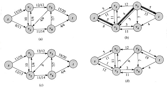
Figure 27.4 (a) The flow network G and flow f of Figure 27.1(b). (b) The residual network Gf with augmenting path p shaded; its residual capacity is cf(p) = c(v2, v3) = 4. (c) The flow in G that results from augmenting along path p by its residual capacity 4. (d) The residual network induced by the flow in (c).
V, we have(f + f')(u, v) = f(u, v) + f'(u, v)
= -f(v, u) - f'(v, u)
= -(f(v, u) + f'(v, u))
= -(f + f')(v, u).
cf(u, v) for all u, v V. By equation (27.5), therefore,(f + f')(u, v) = f(u, v) + f'(u, v)
f(u, v) + (c(u, v) - f(u, v))= c(u, v) .
V - {s, t}, we have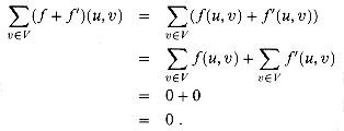
Augmenting paths
cf(p) = min{cf(u, v): (u, v) is on p}. R by
(27.6)
R by â' = â + âp. Then, â' is a flow in G with value | â' | = | â | + |âp| > | â |.Cuts of flow networks
S and t T. (This definition is like the definition of "cut" that we used for minimum spanning trees in Chapter 24, except that here we are cutting a directed graph rather than an undirected graph, and we insist that s S and t T.) If f is a flow, then the net flow across the cut (S, T) is defined to be â(S, T). The capacity of the cut (S, T) is c(S, T).â(v1, v3) + â(v2, v3) + â(v2, v4) = 12 + (-4) + 11
= 19,
c(vl, v3) + c(v2, v4) = 12 + 14
= 26.
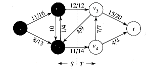
Figure 27.5 A cut (S, T) in the flow network of Figure 27.1(b), where S = {s, v1, v2 } and T = {v3, v4, t}. The vertices in S are black, and the vertices in T are white. The net flow across (S, T) is â(S, T) = 19, and the capacity is c(S, T) = 26.
â(S, T) = â(S, V) - â(S, S)
= â(S, V)
= â(s, V) + â(S - s, V)
= â(s, V)
= | â | .
|â| = â(S, T)
 (2): Suppose for the sake of contradiction that â is a maximum flow in G but that Gâ has an augmenting path p. Then, by Corollary 27.4, the flow sum â + âp, where âp is given by equation (27.6), is a flow in G with value strictly greater than | â |, contradicting the assumption that â is a maximum flow. (3): Suppose that Gâ has no augmenting path, that is, that Gâ contains no path from s to t. Define V : there exists a path from s to
  in Gâ} S trivially and t S because there is no path from s to T in Gâ. For each pair of vertices u and v such that u S and v T, we have â(u, v) = c(u, v), since otherwise (u, v) Eâ and v is in set S. By Lemma 27.5, therefore, | â | = â(S, T) = c(S, T). (1): By Corollary 27.6, | â | c(S, T) for all cuts (S, T). The condition | â | = c(S, T) thus implies that â is a maximum flow.
 The basic Ford-Fulkerson algorithm
E. (In a typical implementation, c(u, v) might be derived from fields stored within vertices and their adjacency lists.) The residual capacity câ(u, v) is computed in accordance with the formula (27.5). The expression câ(p) in the code is actually just a temporary variable that stores the residual capacity of the path p.FORD-FULKERSON(G, s, t)
1 for each edge (u, v)
E[G]2 do â[u, v]
 0
03 â[v, u]
04 while there exists a path p from s to t in the residual network Gâ
5 do câ(p)
min {câ(u, v) : (u, v) is in p}6 for each edge (u, v) in p
7 do â[u, v]
â[u, v]+câ(p)8 â[v, u]
- â[u, v]Analysis of Ford-Fulkerson
 (E). The while loop of lines 4-8 is executed at most | â* | times, since the flow value increases by at least one unit in each iteration. E or (v, u) E}. Edges in the network G are also edges in G', and it is therefore a simple matter to maintain capacities and flows in this data structure. Given a flow â on G, the edges in the residual network Gâ consist of all edges (u, v) of G' such that c(u, v) - â[u, v] 0. The time to find a path in a residual network is therefore O(E') = O(E) if we use either depth-first search or breadth-first search. Each iteration of the while loop thus takes O(E) time, making the total running time of FORD-FULKERSON O(E | â* |).
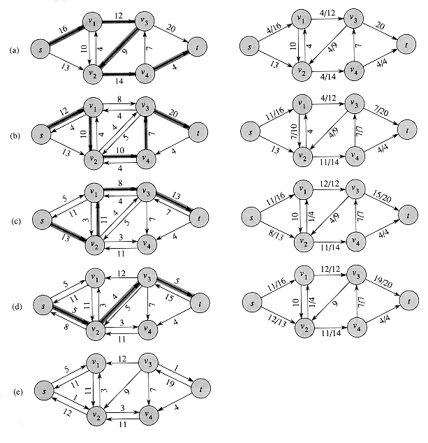
Figure 27.6 The execution of the basic Ford-Fulkerson algorithm. (a)-(d) Successive iterations of the while loop. The left side of each part shows the residual network Gâ from line 4 with a shaded augmenting path p. The right side of each part shows the new flow â that results from adding âp to â. The residual network in (a) is the input network G. (e) The residual network at the last while loop test. It has no augmenting paths, and the flow â shown in (d) is therefore a maximum flow.
Figure 27.7 (a) A flow network for which FORD-FULKERSON can take
(E |â*|) time, where â* is a maximum flow, shown here with | â* | = 2,000,000. An augmenting path with residual capacity 1 is shown. (b) The resulting residual network. Another augmenting path with residual capacity 1 is shown. (c) The resulting residual network. u t, and another 1,000,000 units traverse the path s v t. If the first augmenting path found by FORD-FULKERSON is s u v t, shown in Figure 27.7(a), the flow has value 1 after the first iteration. The resulting residual network is shown in Figure 27.7(b). If the second iteration finds the augmenting path s v u t, as shown in Figure 27.7(b), the flow then has value 2. Figure 27.7(c) shows the resulting residual network. We can continue, choosing the augmenting path s u v t in the odd-numbered iterations and the augmenting path s v u t in the even-numbered iterations. We would perform a total of 2,000,000 augmentations, increasing the flow value by only 1 unit in each.
 (u, v) for the shortest-path distance from u to v in Gf , where each edge has unit distance. V - {s, t}, the shortest-path distance (s, v) in the residual network Gf increases monotonically with each flow augmentation. V - {s, t}, there is a flow augmentation that causes (s, v) to decrease. Let f be the flow just before the augmentation, and let ' be the flow just afterward. Then,'(s, v) < (s, v).'(s, v) '(s, u) for all vertices u V - {s, t} such that '(s, u) < (s, u). Equivalently, we can assume that for all vertices u V - {s, t},'(s, u) < '(s, v) implies (s, u) '(s, u).
(27.7)
' of the form  and consider the vertex u that precedes v on this path. We must have '(s, u) = '(s, v) - 1 by Corollary 25.2, since (u, v) is an edge on p', which is a shortest path from s to v. By our assumption (27.7), therefore,(s, u) '(s, u) .. If â[u, v] < c(u, v), then we have(s, v) (s, u) + 1 (by Lemma 25.3) '(s, u) + 1
=
'(s, v) ,[u, v] = c(u, v), which means (u, v) E. Now, the augmenting path p that was chosen in G to produce G' must contain the edge (v, u) in the direction from v to u, since (u, v) E', (by supposition) and (u, v) E as we have just shown. That is, augmenting flow along the path p pushes flow back along (u, v), and v appears before u on p. Since p is a shortest path from s to t, its subpaths are shortest paths (Lemma 25.1), and thus we have (s, u) = (s, v) + 1. Consequently,(s, v) = (s, u) - 1 '(s, u) - 1=
'(s, v) - 2<
'(s, v) , is critical on an augmenting path p if the residual capacity of p is the residual capacity of (u, v), that is, if c(p) = c(u, v). After we have augmented flow along an augmenting path, any critical edge on the path disappears from the residual network. Moreover, at least one edge on any augmenting path must be critical.(s, v) = (s, u) + 1 .' is the flow in G when this event occurs, then we have'(s, u) = '(s, v) + 1.(s, v) '(s, v) by Lemma 27.8, we have'(s, u) = '(s, v) + 1 (s, v) + 1=
(s, u) + 2. V - 2. Thus, (u, v) can become critical at most O(V) times. Since there are O(E) pairs of vertices that can have an edge between them in a residual graph, the total number of critical edges during the entire execution of the Edmonds-Karp algorithm is O(V E). Each augmenting path has at least one critical edge, and hence the theorem follows.
 Exercises
(u, v) + c(v, u) = c(u, v) + c(v, u).(si,V) = pi. Suppose also that each sink tj consumes exactly qj units, so that (V, tj) = qj, where  ipi = jqj. Show how to convert the problem of finding a flow f that obeys these additional constraints into the problem of finding a maximum flow in a single-source, single-sink flow network.(s, u) and (u, t) change between times at which (u, v) is critical.)
27.3 Maximum bipartite matching
The maximum-bipartite-matching problem
E such that for all vertices v V, at most one edge of M is incident on v. We say that a vertex v V is matched by matching M if some edge in M is incident on v; otherwise, v is unmatched. A maximum matching is a matching of maximum cardinality, that is, a matching M such that for any matching M', we have |M| |M'|. In this section, we shall restrict our attention to finding maximum matchings in bipartite graphs. We assume that the vertex set can be partitioned into V = L R, where L and R are disjoint and all edges in E go between L and R. Figure 27.8 illustrates the notion of a matching.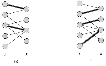
Figure 27.8 A bipartite graph G = (V, E) with vertex partition V = L
R. (a) A matching with cardinality 2. (b) A maximum matching with cardinality 3. L is capable of performing a particular task v R. A maximum matching provides work for as many machines as possible.Finding a maximum bipartite matching
{s, t}. If the vertex partition of G is V = L R, the directed edges of G' are given byE' = {(s, u): u L} {(u, v): u L, v R, and (u, v) E} {(v, t): v R} . on a flow network G = (V, E) is integer-valued if (u, v) is an integer for all (u, v) V  V.
V.
Figure 27.9 The flow network corresponding to a bipartite graph. (a) The bipartite graph G = (V, E) with vertex partition V = L
R from Figure 27.8. A maximum matching is shown by shaded edges. (b) The corresponding flow network G' with a maximum flow shown. Each edge has unit capcity. Shaded edges have a flow of 1, and all other edges carry no flow. The shaded edges from L to R correspond to those in a maximum matching of the bipartite graph. R, and let G'= (V', E') be its corresponding flow network. If M is a matching in G, then there is an integer-valued flow in G' with value |â| = |M|. Conversely, if f is an integer-valued flow in G', then there is a matching M in G with cardinality |M| = |â|. M, then f(s, u) = f(u, v) = f(v, t) = 1 and f(u, s) = f(v, u) = f(t, v) = -1. For all other edges (u, v) E', we define f(u, v) = 0. M corresponds to 1 unit of flow in G' that traverses the path s u v t. Moreover, the paths induced by edges in m are vertex-disjoint, except for s and t. To verify that f indeed satisfies skew symmetry, the capacity constraints, and flow conservation, we need only observe that f can be obtained by flow augmentation along each such path. The new flow across cut (L {s}, R {t}) is equal to |M|; thus, by Lemma 27.5, the value of the flow is |â| = |M|.M = {(u, v): u L, v R, and f(u, v) > 0} . L has only one entering edge, namely (s, u), and its capacity is 1. Thus, each u L has at most one unit of positive net flow entering it. Since f is integer-valued, for each u L, 1 unit of positive net flow enters u if and only if there is exactly one vertex v R such that f(u, v) = 1. Thus, at most one edge leaving each u L carries positive net flow. A symmetric argument can be made for each v R. The set M defined in the statement of the theorem is therefore a matching. L, we have f(s, u) = 1, and for every edge (u, v) E - M, we have f(u,v) = 0. Consequently, using Lemma 27.1, skew symmetry, and there being no edges from L to t, we obtain|M| = â(L,R)
= â(L, V') - â(L, L) - â(L, s) - â(L, t)
= 0 - 0 + â(s, L) - 0
= â(s, V')
= |â| .
Exercises
R, and let G' be its corresponding flow network. Give a good upper bound on the length of any augmenting path found in G' during the execution of FORD-FULKERSON. R, where |L| = |R|. For any X V, define the neighborhood of X asN(X) = {y V : (x, y) E for some x X}, |N(A)| for every subset A L. R, is d-regular if every vertex v V has degree exactly d. Every d-regular bipartite graph has |L| = |R|. Prove that every d-regular bipartite graph has a matching of cardinality |L| by arguing that a minimum cut of the corresponding flow network has capacity |L|.* 27.4 Preflow-push algorithms
R that satisfies skew symmetry, capacity constraints, and the following relaxation of flow conservation: f(V, u) 0 for all vertices u V - {s}. That is, the net flow into each vertex other than the source is nonnegative. We call the net flow into a vertex u the excess flow into u, given bye(u) = f(V, u) .
(27.8)
V - {s, t} is overflowing if e(u) > 0.Intuition
The basic operations
N is a height function if h(s) = |V|,h(t) = 0, and
h(u)
h(v) + 1 Ef . We immediately obtain the following lemma. V, if h(u) > h(v) + 1, then (u, v) is not an edge in the residual graph. PUSH(u, v)
1
 Applies when: u is overflowing, cf [u, v] > 0, and h[u] = h[v] + 1.
2
 Action: Push df (u, v) = min(e[u], cf(u, v)) units of flow
from u to v.
3 df(u, v)
min(e[u], cf(u, v))4 f[u, v]
f[u, v] +df(u, v)5 f[v, u]
- f[u, v]6 e[u]
e[u] -  (u, v)
7 e[v]
e[v] + df(u, v) h[v] for all vertices v. In other words, we can lift an overflowing vertex u if for every vertex v for which there is residual capacity from u to v, flow cannot be pushed from u to v because v is not downhill from u. (Recall that by definition, neither the source s nor the sink t can be overflowing, so neither s nor t can be lifted.)LIFT(u)
1
 Applies when: u is overflowing and for all v V,
(u, v)
Ef implies h[u] h[v].2
 Action: Increase the height of u.
3 h[u]
1 + min {h[v]: (u, v) Ef}câ (u, v) = c(u, v) - f[u, v]
= c(u, v) + f [v, u]
> 0,
Eâ. The operation LIFT(u) thus gives u the greatest height allowed by the constraints on height functions.The generic algorithm
INITIALIZE-PREFLOW(G, s)
1 for each vertex u
V[G]2 do h[u]
03 e[u]
04 for each edge (u, v)
E[G]5 do â[u, v]
06 â[v, u]
07 h[s]
|V[G]|8 for each vertex u
Adj[s]9 do â[s, u]
c(s, u)10 â[u, s]
-c(s, u)11 e[u]
c(s, u)INITIALIZE-PREFLOW creates an initial preflow â defined by
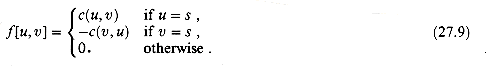
(27.9)
GENERIC-PREFLOW-PUSH(G)
1 INITIALIZE-PREFLOW(G, s)
2 while there exists an applicable push or lift operation
3 do select an applicable push or lift operation and perform it
be a preflow, and let h be any height function for . If u is any overflowing vertex, then either a push or lift operation applies to it. h(v) + 1 because h is a height function. If a push operation does not apply to u, then for all residual edges (u, v), we must have h(u) < h(v) + 1, which implies h(u) h(v) . Thus, a lift operation can be applied to u. Correctness of the preflow-push method
is a maximum flow. We shall later prove that it terminates. We start with some observations about the height function h. V, the height h[u] never decreases. Moreover, whenever a lift operation is applied to a vertex u, its height h[u] increases by at least 1. E, we have h[u] h[v]; this implies that h[u] < 1 + min {h[v]: (u, v) E}, and so the operation must increase h[u]. E that leaves u, then the operation LIFT(u) ensures that h[u] h[v] + 1 afterward. Now consider a residual edge (w, u) that enters u. By Lemma 27.15, h[w] h[u] + 1 before the operation LIFT(u) implies h[w] < h[u] + 1 afterward. Thus, the operation LIFT(u) leaves h a height function., and it may remove (u, v) from E. In the former case, we have h[v] = h[u] - 1, and so h remains a height function. In the latter case, the removal of (u, v) from the residual network removes the corresponding constraint, and h again remains a height function. . v0, v1, . . . , vk
 from s to t in G, where v0 = s and vk = t. Without loss of generality, p is a simple path, and so k < |V|. For i = 0, 1, . . . , k - 1, edge (vi, vi + 1) E Because h is a height function, h(vi) h(vi+1) + 1 for i = 0, 1, . . . , k - 1 . Combining these inequalities over path p yields h(s) h(t) + k. But because h(t) = 0, we have h(s) k < |V| , which contradicts the requirement that h(s) = |V| in a height function. is always a preflow, there are no overflowing vertices. Therefore, is a flow. Because h is a height function, by Lemma 27.17 there is no path from s to t in the residual network G. By the max-flow min-cut theorem, therefore, is a maximum flow.
 Analysis of the preflow-push method
be a preflow in G. Then, for any overflowing vertex u, there is a simple path from u to s in the residual network G.}, and suppose for the sake of contradiction that s U. Let  U and
U and  that (w, v) 0. Why? If (w, v) > 0, then (v, w) < 0, which implies that c(v, w) = c(v, w) - (v, w) > 0. Hence, there exists an edge (v, w) E, and therefore a simple path of the form
  in G, contradicting our choice of w.
 since every term in this implicit summation is nonpositive. Thus, from equation (27.8) and Lemma 27.1, we can conclude that
 V - {s}, we must therefore have e(v) = 0 for all vertices v U. In particular, e(u) = 0, which contradicts the assumption that u is overflowing. 2 |V| - 1 for all vertices u V. V - {s, t}. Lemma 27.19 tells us that there is a simple path p from u to s in G. Let p = v0, v1, . . . , vk, where v0 = u, vk = s, and k |V| - 1 because p is simple. For i = 0, 1, . . . , k - 1, we have (vi, vi + 1) E, and therefore, by Lemma 27.16, h[vi] h[vi+1] + 1. Expanding these inequalities over path p yields h[u] = h[v0] h[vk] + k h[s] + (|V| - 1) = 2 |V| - 1. V - {s, t}. The operation LIFT(u) increases h[u]. The value of h[u] is initially 0 and by Lemma 27.20 grows to at most 2 |V| - 1. Thus, each vertex u V - {s, t} is lifted at most 2 |V| - 1 times, and the total number of lift operations performed is at most (2 |V| - 1)(|V| - 2) < 2 |V|2. V, consider the saturating pushes from u to v and from v to u. If there are any such pushes, at least one of (u, v) and (v, u) is actually an edge in E. Now, suppose that a saturating push from u to v has occurred. In order for another push from u to v to occur later, the algorithm must first push flow from v to u, which cannot happen until h[v] increases by at least 2. Likewise, h[u] must increase by at least 2 between saturating pushes from v to u. 1; thus, the first integer in A is at least 1. When the last such push occurs, we have h[u] + h[v] (2 |V| - 1) + (2 |V| - 2) = 4 |V| - 3 by Lemma 27.20; the last integer in A is thus at most 4 |V| - 3. By the argument from the previous paragraph, at most every other integer can occur in A. Thus, the number of integers in A is at most ((4 |V| - 3) - 1)/2 + 1 = 2 |V| - 1. (We add 1 to make sure that both ends of the sequence are counted.) The total number of saturating pushes between vertices u and v is therefore at most 2 |V| - 1. Multiplying by the number of edges gives a total number of saturating pushes of at most (2 |V| - 1) |E| < 2 |V| |E|. V2 (V + E). = vX h[v], where X V is the set of overflowing vertices. Initially, = 0. Observe that lifting a vertex u increases by at most 2V, since the set over which the sum is taken is the same and u cannot be lifted by more than its maximum possible height, which, by Lemma 27.20, is at most 2V. Also, a saturating push from a vertex u to a vertex v increases by at most 2V, since no heights change and only vertex v, whose height is at most 2V, can possibly become overflowing. Finally, observe that a nonsaturating push from u to v decreases by at least 1, since u is no longer overflowing after the push, v is overflowing afterward even if it wasn't beforehand, and h[v] - h[u] = - 1. is constrained by Corollary 27.21 and Lemma 27.22 to be at most (2V)(2V2) + (2V)(2VE) = 4V2 (V + E). Since 0, the total amount of decrease, and therefore the total number of nonsaturating pushes, is at most 4V2 (V + E).
 Exercises
V, E, and k. (Hint: How many times can each edge support a nonsaturating push before it becomes saturated?)h[s]
V[G] - 2(u, v) be the distance (number of edges) from u to v in the residual network G. Show that GENERIC-PREFLOW-PUSH maintains the properties that h[u] < V implies h[u] (u, t) and that h[u] V implies h[u] - V (u, s). (u, v) be the distance from u to v in the residual network G. Show how the generic preflow-push algorithm can be modified to maintain the property that h[u] < V implies h[u] = (u, t) and that h[u] V implies h[u] - V = (u, s). The total time that your implementation dedicates to maintaining this property should be O(V E).V2 E for V 4.* 27.5 The lift-to-front algorithm
Admissible edges and networks
is a preflow in G, and h is a height function, then we say that (u,v) is an admissible edge if c (u, v) > 0 and h(u) = h(v) + 1. Otherwise, (u, v) is inadmissible. The admissible network is G,h = (V,E,h), where E,h is the set of admissible edges. is a preflow in G, and h is a height function on G, then the admissible network G,h = (V,E,h) is acyclic.,h contains a cycle p = (v0 v1, . . ., vk), where v0 = vk and k > 0. Since each edge in p is admissible, we have h(vi-1) = h(vi) + 1 for i = 1,2, . . ., k. Summing around the cycle gives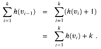 be a preflow in G, and let h be a height function. If a vertex u is overflowing and (u, v) is an admissible edge, then PUSH(u, v) applies. The operation does not create any new admissible edges, but it may cause (u, v) to become inadmissible.(u, v) = 0 afterward and (u, v) becomes inadmissible. be a preflow in G, and let h be a height function. If a vertex u is overflowing and there are no admissible edges leaving u, then LIFT(u) applies. After the lift operation, there is at least one admissible edge leaving u, but there are no admissible edges entering u. E }. Thus, if is a vertex that realizes the minimum in this set, the edge (u,v) becomes admissible. Hence, after the lift, there is at least one admissible edge leaving u.] = h[u] + 1 after the lift, and therefore h[] > h[u] + 1 just before the lift. But by Lemma 27.13, no residual edges exist between vertices whose heights differ by more than 1. Moreover, lifting a vertex does not change the residual network. Thus, (,u) is not in the residual network, and hence it cannot be in the admissible network.
 Neighbor lists
V is a singly linked list of the neighbors of u in G. Thus, vertex appears in the list N[u] if (u,) E or (,u) E. The neighbor list N[u] contains exactly those vertices for which there may be a residual edge (u,). The first vertex in N[u] is pointed to by head [N[u]]. The vertex following in a neighbor list is pointed to by next-neighbor[]; this pointer is NIL if is the last vertex in the neighbor list.Discharging an overflowing vertex
DISCHARGE(u)
1 while e[u] > 0
2 do
current[u]3 if
= NIL4 then LIFT(u)
5 current[u]
head[N[u]]6 elseif c
(u,) > 0 and h[u] = h[] + 17 then PUSH(u,
)8 else current[u]
next-neighbor[] in the neighbor list N[u].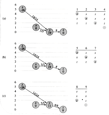
Figure 27.10 Discharging a vertex. It takes 15 iterations of the while loop of DISCHARGE to push all the excess flow from vertex y. Only the neighbors of y and edges entering or leaving y are shown. In each part, the number inside each vertex is its excess at the beginning of the first iteration shown in the part, and each vertex is shown at its height throughout the part. To the right is shown the neighbor list N[y] at the beginning of each iteration, with the iteration number on top. The shaded neighbor is current[y]. (a) Initially, there are 19 units of excess to push from y, and current[y] = s. Iterations 1, 2, and 3 just advance current[y], since there are no admissible edges leaving y. In iteration 4, current[y] = NIL (shown by the shading being below the neighbor list), and so y is lifted and current[y] is reset to the head of the neighbor list. (b) After lifting, vertex y has height 1. In iterations 5 and 6, edges (y, s) and (y, x) are found to be inadmissible, but 8 units of excess flow are pushed from y to z in iteration 7. Because of the push, current[y] is not advanced in this iteration. (c) Because the push in iteration 7 saturated edge (y, z), it is found inadmissible in iteration 8. In iteration 9, current[y] = NIL, and so vertex y is again lifted and current[y] is reset. (d) In iteration 10, (y, s) is inadmissible, but 5 units of excess flow are pushed from y to x in iteration 11. (e) Because current[y] was not advanced in iteration 11, iteration 12 finds (y, x) to be inadmissible. Iteration 13 finds (y, z) inadmissible, and iteration 14 lifts vertex y and resets current[y]. (f) Iteration 15 pushes 6 units of excess flow from y to s. (g) Vertex y now has no excess flow, and DISCHARGE terminates. In this example, DISCHARGE both starts and finishes with the current pointer at the head of the neighbor list, but in general this need not be the case.
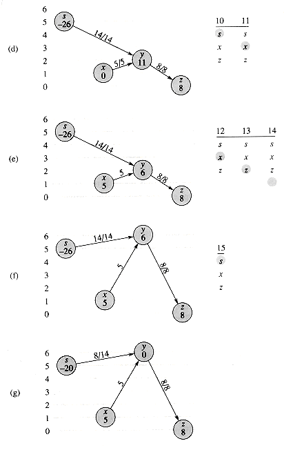 . N[u] during a pass, the edge (u, v) must be deemed inadmissible by the test in line 6. Thus, by the time the pass completes, every edge leaving u has been determined to be inadmissible at some time during the pass. The key observation is that at the end of the pass, every edge leaving u is still inadmissible. Why? By Lemma 27.27, pushes cannot create any admissible edges, let alone one leaving u. Thus, any admissible edge must be created by a lift operation. But the vertex u is not lifted during the pass, and by Lemma 27.28, any other vertex that is lifted during the pass has no entering admissible edges. Thus, at the end of the pass, all edges leaving u remain inadmissible, and the lemma is proved.
 The lift-to-front algorithm
LIFT-TO-FRONT(G, s, t)
1 INITIALIZE-PREFLOW(G, s)
2 L
V[G] - {s, t}, in any order3 for each vertex u
V[G] - {s, t}4 do current[u]
head[N[u]]5 u
head[L]6 while u
NIL7 do old-height
h[u]8 DISCHARGE(u)
9 if h[u] > old-height
10 then move u to the front of list L
11 u
next[u]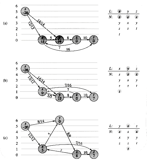
Figure 27.11 The action of LIFT-TO-FRONT. (a) A flow network just before the first iteration of the while loop. Initially, 26 units of flow leave source s. On the right is shown the initial list L =
x, y, z, where initially u = x. Under each vertex in list L is its neighbor list, with the current neighbor shaded. Vertex x is discharged. It is lifted to height 1, 5 units of excess flow are pushed to y, and the 7 remaining units of excess are pushed to the sink t. Because x is lifted, it is moved to the head of L, which in this case does not change the structure of L. (b) After x, the next vertex in L that is discharged is y. Figure 27.10 shows the detailed action of discharging y in this situation. Because y is lifted, it is moved to the head of L. (c) Vertex x now follows y in L, and so it is again discharged, pushing all 5 units of excess flow to t. Because vertex x is not lifted in this discharge operation, it remains in place in list L. (d) Since vertex z follows vertex x in L, it is discharged. It is lifted to height 1 and all 8 units of excess flow are pushed to t. Because z is lifted, it is moved to the front of L. (e) Vertex y now follows vertex z in L and is therefore discharged. But because y has no excess, DISCHARGE immediately returns, and y remains in place in L. Vertex x is then discharged. Because it, too, has no excess, DISCHARGE again returns, and x remains in place in L. LIFT-TO-FRONT has reached the end of list L and terminates. There are no overflowing vertices, and the preflow is a maximum flow. ,h = (V, E,h).V and h[v] = 0 for all v V - {s}. Since |V | 2 (because it contains at least s and t), no edge can be admissible. Thus, E,h =
 , and any ordering of V - {s, t} is a topological sort of G,h.
Analysis
degree(u)) times overall for the vertex. For all vertices, therefore, the total amount of work done in advancing pointers in neighbor lists is O(V E) by the handshaking lemma (Exercise 5.4-1).Exercises
v1, v2, v3, v4 and that the neighbor lists areN[v1] =
s, v2, v3 ,N[v2] =
s, v1, v3, v4 ,N[v3] =
v1, v2, v4, t ,N[v4] =
v2, v3, t . h[u] + 1. How does this change affect the analysis of LIFT-To-FRONT?Problems
Figure 27.12 Grids for the escape problem. Starting points are black, and other grid vertices are white. (a) A grid with an escape, shown by shaded paths. (b) A grid with no escape.
n2 starting points (x1, y1), (x2, y2), . . . , (xm, ym) in the grid, the escape problem is to determine whether or not there are m vertex-disjoint paths from the starting points to any m different points on the boundary. For example, the grid in Figure 27.12(a) has an escape, but the grid in Figure 27.12(b) does not.V' = {x0, x1, . . . , xn} {y0, y1, . . . , yn} ,E' = {(x0, xi) : i V} {(yi, y0) : i V} {(xi, yj) : (i, j) E} ,and run a maximum-flow algorithm.)
I. The cost of carrying instrument Ik is ck dollars. The professor's job is to find an efficient algorithm to determine which experiments to perform and which instruments to carry for a given flight in order to maximize the net revenue, which is the total income from experiments performed minus the total cost of all instruments carried. Rj, then there is an edge (Ik, Ej) of infinite capacity. T for a finite-capacity cut (S, T) of G, then Ik T for each Ik Rj. .
.