


B-trees are balanced search trees designed to work well on magnetic disks or other direct-access secondary storage devices. B-trees are similar to red-black trees (Chapter 14), but they are better at minimizing disk I/O operations.
B-trees differ significantly from red-black trees in that B-tree nodes may have many children, from a handful to thousands. That is, the "branching factor" of a B-tree can be quite large, although it is usually determined by characteristics of the disk unit used. B-trees are similar to red-black trees in that every n-node B-tree has height O(lg n), although the height of a B-tree can be considerably less than that of a red-black tree because its branching factor can be much larger. Therefore, B-trees can also be used to implement many dynamic-set operations in time O(lg n).
B-trees generalize binary search trees in a natural manner. Figure 19.1 shows a simple B-tree. If a B-tree node x contains n[x] keys, then x has n[x] + 1 children. The keys in node x are used as dividing points separating the range of keys handled by x into n[x] + 1 subranges, each handled by one child of x. When searching for a key in a B-tree, we make an (n[x] + 1)-way decision based on comparisons with the n[x] keys stored at node x.
Section 19.1 gives a precise definition of B-trees and proves that the height of a B-tree grows only logarithmically with the number of nodes it contains. Section 19.2 describes how to search for a key and insert a key into a B-tree, and Section 19.3 discusses deletion. Before proceeding, however, we need to ask why data structures designed to work on a magnetic disk are evaluated differently than data structures designed to work in main random-access memory.
Data structures on secondary storage
There are many different technologies available for providing memory capacity in a computer system. The primary memory (or main memory) of a computer system typically consists of silicon memory chips, each of which can hold 1 million bits of data. This technology is more expensive per bit stored than magnetic storage technology, such as tapes or disks. A typical computer system has secondary storage based on magnetic disks; the amount of such secondary storage often exceeds the amount of primary memory by several orders of magnitude.
Figure 19.2 shows a typical disk drive. The disk surface is covered with a magnetizable material. The read/write head can read or write data magnetically on the rotating disk surface. The read/write arm can position the head at different distances from the center of the disk. When the head is stationary, the surface that passes underneath it is called a track. Theinformation stored on each track is often divided into a fixed number of equal-sized pages; for a typical disk, a page might be 2048 bytes in length.The basic unit of information storage and retrieval is usually a page of information--that is, disk reads and writes are typically of entire pages.The access time--the time required to position the read/write head and to wait for a given page of information to pass underneath the head--may be large (e.g., 20 milliseconds), while the time to read or write a page, once accessed, is small. The price paid for the low cost of magnetic storage techniques is thus the relatively long time it takes to access the data. Since moving electrons is much easier than moving large (or even small) objects, storage devices that are entirely electronic, such as silicon memory chips, have a much smaller access time than storage devices that have moving parts, such as magnetic disk drives. However, once everything is positioned correctly, reading or writing a magnetic disk is entirely electronic (aside from the rotation of the disk), and large amounts of data can be read or written quickly.
Often, it takes more time to access a page of information and read it from a disk than it takes for the computer to examine all the information read. For this reason, in this chapter we shall look separately at the two principal components of the running time:
The number of disk accesses is measured in terms of the number of pages of information that need to be read from or written to the disk. We note that disk access time is not constant--it depends on the distance between the current track and the desired track and also on the initial rotational state of the disk. We shall nonetheless use the number of pages read or written as a crude first-order approximation of the total time spent accessing the disk.
In a typical B-tree application, the amount of data handled is so large that all the data do not fit into main memory at once. The B-tree algorithms copy selected pages from disk into main memory as needed and write back onto disk pages that have changed. Since the B-tree algorithms only need a constant number of pages in main memory at any time, the size of main memory does not limit the size of B-trees that can be handled.
We model disk operations in our pseudocode as follows. Let x be a pointer to an object. If the object is currently in the computer's main memory, then we can refer to the fields of the object as usual: key[x], for example. If the object referred to by x resides on disk, however, then we must perform the operation DISK-READ(x) to read object x into main memory before its fields can be referred to. (We assume that if x is already in main memory, then DISK-READ(x) requires no disk accesses; it is a "noop.") Similarly, the operation DISK-WRITE(x) is used to save any changes that have been made to the fields of object x. That is, the typical pattern for working with an object is as follows.
The system can only keep a limited number of pages in main memory at any one time. We shall assume that pages no longer in use are flushed from main memory by the system; our B-tree algorithms will ignore this issue.
Since in most systems the running time of a B-tree algorithm is determined mainly by the number of DISK-READ and DISK-WRITE operations it performs, it is sensible to use these operations intensively by having them read or write as much information as possible. Thus, a B-tree node is usually as large as a whole disk page. The number of children a B-tree node can have is therefore limited by the size of a disk page.
For a large B-tree stored on a disk, branching factors between 50 and 2000 are often used, depending on the size of a key relative to the size of a page. A large branching factor dramatically reduces both the height of the tree and the number of disk accesses required to find any key. Figure 19.3 shows a B-tree with a branching factor of 1001 and height 2 that can store over one billion keys; nevertheless, since the root node can be kept permanently in main memory, only two disk accesses at most are required to find any key in this tree!
To keep things simple, we assume, as we have for binary search trees and red-black trees, that any "satellite information" associated with a key is stored in the same node as the key. In practice, one might actually store with each key just a pointer to another disk page containing the satellite information for that key. The pseudocode in this chapter implicitly assumes that the satellite information associated with a key, or the pointer to such satellite information, travels with the key whenever the key is moved from node to node. Another commonly used B-tree organization stores all the satellite information in the leaves and only stores keys and child pointers in the internal nodes, thus maximizing the branching factor of the internal nodes.
A B-tree T is a rooted tree (with root root[T]) having the following properties.
1. Every node x has the following fields:
a. n[x], the number of keys currently stored in node x,
b. the n[x] keys themselves, stored in nondecreasing order: key1[x]
c. leaf [x], a boolean value that is TRUE if x is a leaf and FALSE if x is an internal node.
2. If x is an internal node, it also contains n[x] + 1 pointers c1 [x], c2[x], . . . , cn[x]+1[x] to its children. Leaf nodes have no children, so their ci fields are undefined.
3. The keys keyi[x] separate the ranges of keys stored in each subtree: if ki is any key stored in the subtree with root ci[x], then
4. Every leaf has the same depth, which is the tree's height h.
5. There are lower and upper bounds on the number of keys a node can contain. These bounds can be expressed in terms of a fixed integer t
a. Every node other than the root must have at least t - 1 keys. Every internal node other than the root thus has at least t children. If the tree is nonempty, the root must have at least one key.
b. Every node can contain at most 2t - 1 keys. Therefore, an internal node can have at most 2t children. We say that a node is full if it contains exactly 2t - 1 keys.
The simplest B-tree occurs when t = 2. Every internal node then has either 2, 3, or 4 children, and we have a 2-3-4 tree. In practice, however, much larger values of t are typically used.
The number of disk accesses required for most operations on a B-tree is proportional to the height of the B-tree. We now analyze the worst-case height of a B-tree.
Theorem 19.1
If n
Proof If a B-tree has height h, the number of its nodes is minimized when the root contains one key and all other nodes contain t - 1 keys. In this case, there are 2 nodes at depth 1, 2t nodes at depth 2, 2t2 nodes at depth 3, and so on, until at depth h there are 2th-1 nodes. Figure 19.4 illustrates such a tree for h = 3. Thus, the number n of keys satisfies the inequality
which implies the theorem.
Here we see the power of B-trees, as compared to red-black trees. Although the height of the tree grows as O(lg n) in both cases (recall that t is a constant), for B-trees the base of the logarithm can be many times larger. Thus, B-trees save a factor of about lg t over red-black trees in the number of nodes examined for most tree operations. Since examining an arbitrary node in a tree usually requires a disk access, the number of disk accesses is substantially reduced.
19.1-1
Why don't we allow a minimum degree of t = 1?
19.1-2
For what values of t is the tree of Figure 19.1 a legal B-tree?
19.1-3
Show all legal B-trees of minimum degree 2 that represent {1, 2, 3, 4, 5}.
19.1-4
Derive a tight upper bound on the number of keys that can be stored in a B-tree of height h as a function of the minimum degree t.
19.1-5
Describe the data structure that would result if each black node in a red-black tree were to absorb its red children, incorporating their children with its own.
In this section, we present the details of the operations B-TREE-SEARCH, B-TREE-CREATE, and B-TREE-INSERT. In these procedures, we adopt two conventions:
The procedures we present are all "one-pass" algorithms that proceed downward from the root of the tree, without having to back up.
Searching a B-tree is much like searching a binary search tree, except that instead of making a binary, or "two-way," branching decision at each node, we make a multiway branching decision according to the number of the node's children. More precisely, at each internal node x, we make an (n[x] + 1)-way branching decision.
B-TREE-SEARCH is a straightforward generalization of the TREE-SEARCH procedure defined for binary search trees. B-TREE-SEARCH takes as input a pointer to the root node x of a subtree and a key k to be searched for in that subtree. The top-level call is thus of the form B-TREE-SEARCH(root[T], k). If k is in the B-tree, B-TREE-SEARCH returns the ordered pair (y,i) consisting of a node y and an index i such that keyi[y] = k. Otherwise, the value NIL is returned.
Using a linear-search procedure, lines 1-3 find the smallest i such that k
Figure 19.1 illustrates the operation of B-TREE-SEARCH; the lightly shaded nodes are examined during a search for the key R.
As in the TREE-SEARCH procedure for binary search trees, the nodes encountered during the recursion form a path downward from the root of the tree. The number of disk pages accessed by B-TREE-SEARCH is therefore
To build a B-tree T, we first use B-TREE-CREATE to create an empty root node and then call B-TREE-INSERT to add new keys. Both of these procedures use an auxiliary procedure ALLOCATE-NODE, which allocates one disk page to be used as a new node in O(1) time. We can assume that a node created by ALLOCATE-NODE requires no DISK-READ, since there is as yet no useful information stored on the disk for that node.
B-TREE-CREATE requires O(1) disk operations and O(1) CPU time.
Inserting a key into a B-tree is significantly more complicated than inserting a key into a binary search tree. A fundamental operation used during insertion is the splitting of a full node y (having 2t - 1 keys) around its median key keyt[y] into two nodes having t - 1 keys each. The median key moves up into y's parent--which must be nonfull prior to the splitting of y--to identify the dividing point between the two new trees; if y has no parent, then the tree grows in height by one. Splitting, then, is the means by which the tree grows.
The procedure B-TREE-SPLIT-CHILD takes as input a nonfull internal node x (assumed to be in main memory), an index i, and a node y such that y = ci[x] is a full child of x. The procedure then splits this child in two and adjusts x so that it now has an additional child.
Figure 19.5 illustrates this process. The full node y is split about its median key S, which is moved up into y's parent node x. Those keys in y that are greater than the median key are placed in a new node z, which is made a new child of x.
B-TREE-SPLIT-CHILD works by straightforward "cutting and pasting. " Here, y is the ith child of x and is the node being split. Node y originally has 2t - 1 children but is reduced to t - 1 children by this operation. Node z "adopts" the t - 1 largest children of y, and z becomes a new child of x, positioned just after y in x's table of children. The median key of y moves up to become the key in x that separates y and z.
Lines 1-8 create node z and give it the larger t - 1 keys and corresponding t children of y. Line 9 adjusts the key count for y. Finally, lines 10-16 insert z as a child of x, move the median key from y up to x in order to separate y from z, and adjust x's key count. Lines 17-19 write out all modified disk pages. The CPU time used by B-TREE-SPLIT-CHILD is
Inserting a key k into a B-tree T of height h is done in a single pass down the tree, requiring O(h) disk accesses. The CPU time required is O(th) = O(t logt n). The B-TREE-INSERT procedure uses B-TREE-SPLIT-CHILD to guarantee that the recursion never descends to a full node.
Lines 3-9 handle the case in which the root node r is full: the root is split and a new node s (having two children) becomes the root. Splitting the root is the only way to increase the height of a B-tree. Figure 19.6 illustrates this case. Unlike a binary search tree, a B-tree increases in height at the top instead of at the bottom. The procedure finishes by calling B-TREE-INSERT-NONFULL to perform the insertion of key k in the tree rooted at the nonfull root node. B-TREE-INSERT-NONFULL recurses as necessary down the tree, at all times guaranteeing that the node to which it recurses is not full by calling B-TREE-SPLIT-CHILD as necessary.
The auxiliary recursive procedure B-TREE-INSERT-NONFULL inserts key k into node x, which is assumed to be nonfull when the procedure is called. The operation of B-TREE-INSERT and the recursive operation of B-TREE-INSERT-NONFULL guarantee that this assumption is true.
The B-TREE-INSERT-NONFULL procedure works as follows. Lines 3-8 handle the case in which x is a leaf node by inserting key k into x. If x is not a leaf node, then we must insert k into the appropriate leaf node in the subtree rooted at internal node x. In this case, lines 9-11 determine the child of x to which the recursion descends. Line 13 detects whether the recursion would descend to a full child, in which case line 14 uses B-TREE-SPLIT-CHILD to split that child into two nonfull children, and lines 15-16 determine which of the two children is now the correct one to descend to. (Note that there is no need for a DISK-READ(ci[x]) after line 16 increments i, since the recursion will descend in this case to a child that was just created by B-TREE-SPLIT-CHILD.) The net effect of lines 13-16 is thus to guarantee that the procedure never recurses to a full node. Line 17 then recurses to insert k into the appropriate subtree. Figure 19.7 illustrates the various cases of inserting into a B-tree.
The number of disk accesses performed by B-TREE-INSERT is O(h) for a B-tree of height h, since only O(1) DISK-READ and DISK-WRITE operations are performed between calls to B-TREE-INSERT-NONFULL. The total CPU time used is O(th) = O(t1ogt n). Since B-TREE-INSERT-NONFULL is tail-recursive, it can be alternatively implemented as a while loop, demonstrating that the number of pages that need to be in main memory at any time is O(1).
19.2-1
Show the results of inserting the keys
in order into an empty B-tree. Only draw the configurations of the tree just before some node must split, and also draw the final configuration.
19.2-2
Explain under what circumstances, if any, redundant DISK-READ or DISK-WRITE operations are performed during the course of executing a call to B-TREE-INSERT. (A redundant DISK-READ is a DISK-READ for a page that is already in memory. A redundant DISK-WRITE writes to disk a page of information that is identical to what is already stored there.)
19.2-3
Explain how to find the minimum key stored in a B-tree and how to find the predecessor of a given key stored in a B-tree.
19.2-4
Suppose that the keys {1, 2, . . . , n} are inserted into an empty B-tree with minimum degree 2. How many nodes does the final B-tree have?
19.2-5
Since leaf nodes require no pointers to children, they could conceivably use a different (larger) t value than internal nodes for the same disk page size. Show how to modify the procedures for creating and inserting into a B-tree to handle this variation.
19.2-6
Suppose that B-TREE-SEARCH is implemented to use binary search rather than linear search within each node. Show that this makes the CPU time required O(lg n), independently of how t might be chosen as a function of n.
19.2-7
Suppose that disk hardware allows us to choose the size of a disk page arbitrarily, but that the time it takes to read the disk page is a + bt, where a and b are specified constants and t is the minimum degree for a B-tree using pages of the selected size. Describe how to choose t so as to minimize (approximately) the B-tree search time. Suggest an optimal value of t for the case in which a = 30 milliseconds and b = 40 microseconds.
Deletion from a B-tree is analogous to insertion but a little more complicated. We sketch how it works instead of presenting the complete pseudocode.
Assume that procedure B-TREE-DELETE is asked to delete the key k from the subtree rooted at x. This procedure is structured to guarantee that whenever B-TREE-DELETE is called recursively on a node x, the number of keys in x is at least the minimum degree t. Note that this condition requires one more key than the minimum required by the usual B-tree conditions, so that sometimes a key may have to be moved into a child node before recursion descends to that child. This strengthened condition allows us to delete a key from the tree in one downward pass without having to "back up" (with one exception, which we'll explain). The following specification for deletion from a B-tree should be interpreted with the understanding that if it ever happens that the root node x becomes an internal node having no keys, then x is deleted and x's only child c1[x] becomes the new root of the tree, decreasing the height of the tree by one and preserving the property that the root of the tree contains at least one key (unless the tree is empty).
Figure 19.8 illustrates the various cases of deleting keys from a B-tree.
1. If the key k is in node x and x is a leaf, delete the key k from x.
2. If the key k is in node x and x is an internal node, do the following.
a. If the child y that precedes k in node x has at least t keys, then find the predecessor k' of k in the subtree rooted at y. Recursively delete k', and replace k by k' in x. (Finding k' and deleting it can be performed in a single downward pass.)
b. Symmetrically, if the child z that follows k in node x has at least t keys, then find the successor k' of k in the subtree rooted at z. Recursively delete k', and replace k by k' in x. (Finding k' and deleting it can be performed in a single downward pass.)
c. Otherwise, if both y and z have only t- 1 keys, merge k and all of z into y, so that x loses both k and the pointer to z, and y now contains 2t - 1 keys. Then, free z and recursively delete k from y.
3. If the key k is not present in internal node x, determine the root ci[x] of the appropriate subtree that must contain k, if k is in the tree at all. If ci[x] has only t - 1 keys, execute step 3a or 3b as necessary to guarantee that we descend to a node containing at least t keys. Then, finish by recursing on the appropriate child of x.
a. If ci[x] has only t - 1 keys but has a sibling with t keys, give ci[x] an extra key by moving a key from x down into ci[x], moving a key from ci[x]'s immediate left or right sibling up into x, and moving the appropriate child from the sibling into ci[x].
b. If ci[x] and all of ci[x]'s siblings have t - 1 keys, merge ci with one sibling, which involves moving a key from x down into the new merged node to become the median key for that node.
Since most of the keys in a B-tree are in the leaves, we may expect that in practice, deletion operations are most often used to delete keys from leaves. The B-TREE-DELETE procedure then acts in one downward pass through the tree, without having to back up. When deleting a key in an internal node, however, the procedure makes a downward pass through the tree but may have to return to the node from which the key was deleted to replace the key with its predecessor or successor (cases 2a and 2b).
Although this procedure seems complicated, it involves only O(h) disk operations for a B-tree of height h, since only O(1) calls to DISK-READ and DISK-WRITE are made between recursive invocations of the procedure. The CPU time required is O(th) = O(t logt n).
19.3-1
Show the results of deleting C, P, and V, in order, from the tree of Figure 19.8(f).
19.3-2
Write pseudocode for B-TREE-DELETE.
19-1 Stacks on secondary storage
Consider implementing a stack in a computer that has a relatively small amount of fast primary memory and a relatively large amount of slower disk storage. The operations PUSH and POP are supported on single-word values. The stack we wish to support can grow to be much larger than can fit in memory, and thus most of it must be stored on disk.
A simple, but inefficient, stack implementation keeps the entire stack on disk. We maintain in memory a stack pointer, which is the disk address of the top element on the stack. If the pointer has value p, the top element is the (p mod m)th word on page
To implement the PUSH operation, we increment the stack pointer, read the appropriate page into memory from disk, copy the element to be pushed to the appropriate word on the page, and write the page back to disk. A POP operation is similar. We decrement the stack pointer, read in the appropriate page from disk, and return the top of the stack. We need not write back the page, since it was not modified.
Because disk operations are relatively expensive, we use the total number of disk accesses as a figure of merit for any implementation. We also count CPU time, but we charge
a. Asymptotically, what is the worst-case number of disk accesses for n stack operations using this simple implementation? What is the CPU time for n stack operations? (Express your answer in terms of m and n for this and subsequent parts.)
Now, consider a stack implementation in which we keep one page of the stack in memory. (We also maintain a small amount of memory to keep track of which page is currently in memory.) We can perform a stack operation only if the relevant disk page resides in memory. If necessary, the page currently in memory can be written to the disk and the new page read in from the disk to memory. If the relevant disk page is already in memory, then no disk accesses are required.
b. What is the worst-case number of disk accesses required for n PUSH operations? What is the CPU time?
c. What is the worst-case number of disk accesses required for n stack operations? What is the CPU time?
Suppose that we now implement the stack by keeping two pages in memory (in addition to a small number of words for bookkeeping).
d. Describe how to manage the stack pages so that the amortized number of disk accesses for any stack operation is O(1/m) and the amortized CPU time for any stack operation is O(1).
19-2 Joining and splitting 2-3-4 trees
The join operation takes two dynamic sets S' and S\" and an element x such that for any x'
a. Show how to maintain, for every node x of a 2-3-4 tree, the height of the subtree rooted at x as a field height[x]. Make sure that your implementation does not affect the asymptotic running times of searching, insertion, and deletion.
b. Show how to implement the join operation. Given two 2-3-4 trees T' and T\" and a key k, the join should run in O(|h'- h\"|) time, where h' and h\" are the heights of T' and T\", respectively.
c. Consider the path p from the root of a 2-3-4 tree T to a given key k, the set S' of keys in T that are less than k, and the set S\" of keys in T that are greater than k. Show that p breaks S' into a set of trees { T'0,T'1, . . . ,T'm } and a set of keys {k'1,k'2, . . . , k'm}, where, for i = 1, 2, . . . ,m, we have y < k'1 < z for any keys y
d. Show how to implement the split operation on T. Use the join operation to assemble the keys in S' into a single 2-3-4 tree T' and the keys in S\" into a single 2-3-4 tree T\". The running time of the split operation should be O(lg n), where n is the number of keys in T. (Hint: The costs for joining should telescope.)
Knuth [123], Aho, Hopcroft, and Ullman [4], and Sedgewick [175] give further discussions of balanced-tree schemes and B-trees. Comer [48] provides a comprehensive survey of B-trees. Guibas and Sedgewick [93] discuss the relationships among various kinds of balanced-tree schemes, including red-black trees and 2-3-4 trees.
In 1970, J. E. Hopcroft invented 2-3 trees, a precursor to B-trees and 2-3-4 trees, in which every internal node has either two or three children. B-trees were introduced by Bayer and McCreight in 1972 [18]; they did not explain their choice of name.
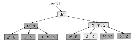
Figure 19.1 A B-tree whose keys are the consonants of English. An internal node x containing n[x] keys has n[x] + 1 children. All leaves are at the same depth in the tree. The lightly shaded nodes are examined in a search for the letter R.
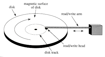
Figure 19.2 A typical disk drive.
 the number of disk accesses, and the CPU (computing) time.
1 . . .
2 x
 a pointer to some object
3 DISK-READ(x)
4 operations that access and/or modify the fields of x
5 DISK-WRITE(x)
 Omitted if no fields of x were changed.
6 other operations that access but do not modify fields of x
7 ...

Figure 19.3 A B-tree of height 2 containing over one billion keys. Each internal node and leaf contains 1000 keys. There are 1001 nodes at depth 1 and over one million leaves at depth 2. Shown inside each node x is n[x], the number of keys in x.
19.1 Definition of B-trees
 key2[x]
  keyn[x][x], and
k1
key1[x] k2 key2[x] keyn[x][x] kn[x]+1 . 2 called the minimum degree of the B-tree:
The height of a B-tree
1, then for any n-key B-tree T of height h and minimum degree t 2,
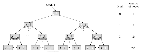
Figure 19.4 A B-tree of height 3 containing a minimum possible number of keys. Shown inside each node x is n[x].

Exercises
19.2 Basic operations on B-trees
The root of the B-tree is always in main memory, so that a DISK-READ on the root is never required; a DISK-WRITE of the root is required, however, whenever the root node is changed. Any nodes that are passed as parameters must already have had a DISK-READ operation performed on them.Searching a B-tree
B-TREE-SEARCH(x, k)
1 i
12 while i
n[x] and k keyi[x]3 do i
i + 14 if i
n[x] and k = keyi[x]5 then return (x, i)
6 if leaf [x]
7 then return NIL
8 else DISK-READ(ci[x])
9 return B-TREE-SEARCH(ci[x], k)
keyi[x], or else they set i to n[x] + 1. Lines 4-5 check to see if we have now discovered the key, returning if we have. Lines 6-9 either terminate the search unsuccessfully (if x is a leaf) or recurse to search the appropriate subtree of x, after performing the necessary DISK-READ on that child. (h) = (logt n), where h is the height of the B-tree and n is the number of keys in the B-tree. Since n[x] < 2t, the time taken by the while loop of lines 2-3 within each node is O(t), and the total CPU time is O(th) = O(t logt n).
Creating an empty B-tree
B-TREE-CREATE(T)
1 x
ALLOCATE-NODE()2 leaf[x]
TRUE3 n[x]
04 DISK-WRITE(x)
5 root[T]
x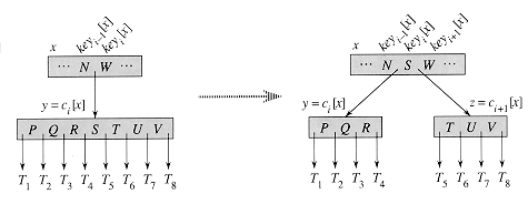
Figure 19.5 Splitting a node with t = 4. Node y is split into two nodes, y and z, and the median key S of y is moved up into y's parent.
Splitting a node in a B-tree
B-TREE-SPLIT-CHILD(x,i,y)
1 z
ALLOCATE-NODE()2 leaf[z]
leaf[y]3 n[z]
t - 14 for j
1 to t - 15 do keyj[z]
keyj+t[y]6 if not leaf [y]
7 then for j
1 to t8 do cj[z]
cj+t[y]9 n[y]
t - 110 for j
n[x] + 1 downto i + 111 do cj+1[x]
cj[x]12 ci+1[x]
z13 for j
n[x] downto i14 do keyj+1[x]
keyj[x]15 keyi[x]
keyt[y]16 n[x]
n[x] + 117 DISK-WRITE(y)
18 DISK-WRITE(z)
19 DISK-WRITE(x)
(t), due to the loops on lines 4-5 and 7-8. (The other loops run for at most t iterations.)Inserting a key into a B-tree
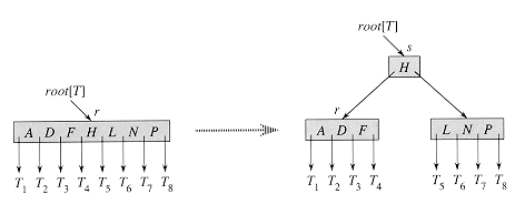
Figure 19.6 Splitting the root with t = 4. Root node r is split in two, and a new root node s is created. The new root contains the median key of r and has the two halves of r as children. The B-tree grows in height by one when the root is split.
B-TREE-INSERT(T,k)
1 r
root[T]2 if n[r] = 2t - 1
3 then s
ALLOCATE-NODE()4 root[T]
s5 leaf[s]
FALSE6 n[s]
07 c1[s]
r8 B-TREE-SPLIT-CHILD(s,1,r)
9 B-TREE-INSERT-NONFULL(s,k)
10 else B-TREE-INSERT-NONFULL(r,k)
B-TREE-INSERT-NONFULL(x,k)
1 i
n[x]2 if leaf[x]
3 then while i
1 and k < keyi[x]4 do keyi+1 [x]
keyi[x]5 i
i - 16 keyi+1[x]
k7 n[x]
n[x] + 18 DISK-WRITE(x)
9 else while i
1 and k < keyi[x]10 do i
i - 111 i
i + 112 DISK-READ(ci[x])
13 if n[ci[x]] = 2t - 1
14 then B-TREE-SPLIT-CHILD(x,i,ci[x])
15 if k > keyi[x]
16 then i
i + 117 B-TREE-INSERT-NONFULL(ci[x],k)
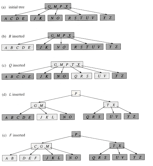
Figure 19.7 Inserting keys into a B-tree. The minimum degree t for this B-tree is 3, so a node can hold at most 5 keys. Nodes that are modified by the insertion process are lightly shaded. (a) The initial tree for this example. (b) The result of inserting B into the initial tree; this is a simple insertion into a leaf node. (c) The result of inserting Q into the previous tree. The node RSTUV is split into two nodes containing RS and UV, the key T is moved up to the root, and Q is inserted in the leftmost of the two halves (the RS node). (d) The result of inserting L into the previous tree. The root is split right away, since it is full, and the B-tree grows in height by one. Then L is inserted into the leaf containing JK. (e) The result of inserting F into the previous tree. The node ABCDE is split before F is inserted into the rightmost of the two halves (the DE node).
Exercises
F, S, Q, K, C, L, H, T, V, W, M, R, N, P, A, B, X, Y, D, Z, E
19.3 Deleting a key from a B-tree

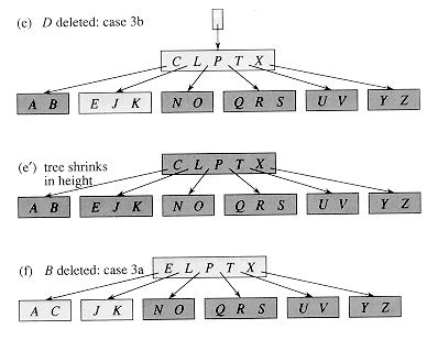
Figure 19.8 Deleting keys from a B-tree. The minimum degree for this B-tree is t = 3, so a node (other than the root) cannot have less than 2 keys. Nodes that are modified are lightly shaded. (a) The B-tree of Figure 19.7(e). (b) Deletion of F. This is case 1: simple deletion from a leaf. (c) Deletion of M. This is case 2a: the predecessor L of M is moved up to take M's position. (d) Deletion of G. This is case 2c: G is pushed down to make node DEGJK, and then G is deleted from this leaf (case 1). (e) Deletion of D. This is case 3b: the recursion can't descend to node CL because it has only 2 keys, so P is pushed down and merged with CL and TX to form CLPTX; then, D is deleted from a leaf (case 1). (e') After (d), the root is deleted and the tree shrinks in height by one. (f) Deletion of B. This is case 3a: C is moved to fill B's position and E is moved to fill C's position.
Exercises
Problems
 p/m
p/m of the disk, where m is the number of words per page.(m) for any disk access to a page of m words.
 S' and x\" S\", we have key[x'] < key[x] < key[x\"]. It returns a set S = S'
  {x} S\". The split operation is like an "inverse" join: given a dynamic set S and an element x S, it creates a set S' consisting of all elements in S - {x} whose keys are less than key[x] and a set S\" consisting of all elements in S - {x} whose keys are greater than key[x]. In this problem, we investigate how to implement these operations on 2-3-4 trees. We assume for convenience that elements consist only of keys and that all key values are distinct. T'i-1 and z T'i. What is the relationship between the heights of T'i-1 and T'i? Describe how p breaks S\" into sets of trees and keys.
Chapter notes